Similar articles

Abstract: The Hong Kong Observatory (HKO) provides low-level turbulence alerting service for the Hong Kong International Airport (HKIA) through the windshear and turbulence warning system (WTWS). In the WTWS, turbulence intensities along the flight paths of the airport are estimated based upon correlation equations established between the surface anemometer data and the turbulence data from research aircraft before the opening of the airport. The research aircraft data are not available on day-to-day basis. The remote sensing meteorological instruments, such as the Doppler light detection and ranging (LIDAR) and radar, may be used to provide direct measurements of turbulence intensities over the runway corridors. The performances of LIDAR- and radar-based turbulence intensity data are studied in this paper based on actual turbulence intensity measurements made on 423 commercial jets for a typical case of terrain-induced turbulence in association with a typhoon. It turns out that, with the tuning of the relative operating characteristic (ROC) curve between hit rate and false alarm rate, the LIDAR-based turbulence intensity measurement performs better than the anemometer-based estimation of WTWS for turbulence intensity at moderate level or above. On the other hand, the radar-based measurement does not perform as well when compared with WTWS. By combining LIDAR- and radar-based measurements, the performance is slightly better than WTWS, mainly as a result of contribution from LIDAR-based measurement. As a result, the LIDAR-based turbulence intensity measurement could be used to replace anemometer-based estimate for non-rainy weather conditions. Further enhancements of radar-based turbulence intensity measurement in rain would be necessary.

1.  Introduction

 The Hong Kong International Airport (HKIA), China is situated in an area of complex terrain. To its south is the mountainous Lantau Island, with peaks rising to about 1000 m above mean sea level with valleys as low as 400 m. Terrain-disrupted airflow disturbances may occur inside and around HKIA with prevailing easterly through southeasterly to southwesterly winds. They may lead to significant turbulence to be encountered by the landing and departing aircraft.

 The Hong Kong Observatory (HKO) provides low-level turbulence alerting service for the aircraft at HKIA. In accordance with the standard of International Civil Aviation Organization (ICAO), turbulence for aviation meteorology is quantified in terms of the cube root of eddy dissipation rate (EDR^1/3) (ICAO, 2010). For low-level turbulence, i.e., turbulence encountered by the aircraft within a range of 3 nautical miles (1 nautical mile=1853 m) from the runway end, it is considered to be significant if the turbulence is moderate (EDR^1/3=0.3–0.5 m^2/3·s⁻¹) or severe (EDR^1/3>0.5 m^2/3·s⁻¹). At HKIA, significant turbulence on average occurs at a frequency of once every 2000 flights (HKO, IFALPA and GAPAN, 2010).

 Turbulence alerting service for HKIA is provided by HKO through the use of windshear and turbulence warning system (WTWS). In this system, turbulence intensities along the flight paths of HKIA are given based on correlation equations established between the turbulence intensities measured by research aircraft and surface anemometer readings in Hong Kong through field studies conducted before the opening of HKIA in 1998. As such, turbulence intensities are not measured directly at the flight paths in day-to-day operations.

 The use of remote sensing meteorological instruments at HKIA offers the possibility of measuring the turbulence intensities directly at the flight paths. Such instruments include the Doppler light detection and ranging (LIDAR) systems for non-rainy weather conditions, and terminal Doppler weather radar (TDWR) in rain. The setup of the meteorological instruments at HKIA is shown in Fig. 1.




 There are some previous studies of the application of remote sensing instruments for turbulence intensity measurements at HKIA. In (Chan and Mok, 2004), turbulent airflow during Typhoon Imbudo in 2003 was studied by considering flight data and spectrum width data of the LIDAR. A total of 82 sets of flight data are considered in this typhoon episode and the study suggests that the LIDAR could be useful in turbulence detection. Another study on the comparison between LIDAR-based EDR and WTWS EDR had been made by Chan (2010) for a number of cases of turbulent airflow at HKIA, including a tropical cyclone case. This is a preliminary study to examine the performance of the various EDR values based on limited number of pilot reports of significant turbulence.

 In the present study, a much larger sample size of 423 sets of flight data is considered to cover another case of turbulent airflow at HKIA brought about by a tropical cyclone: Typhoon Nesat in 2011. The larger dataset is used to establish the robustness of turbulence alerting service using the data from the remote sensing meteorological instruments (namely, LIDAR and TDWR) in comparison with the existing service provided by WTWS using anemometer-based measurements. Moreover, instead of directly using the spectrum width data from the LIDAR as shown in (Chan and Mok, 2004), which is subject to contamination of the turbulence signature by large-scale windshear, the structure function approach of LIDAR EDR calculations as shown in (Chan, 2010) would be adopted. In addition to a larger sample size, an objectively determined EDR from quick access recorder (QAR) data from the aircraft is used to gauge the performance of various EDR values instead of the pilot reports used in (Chan, 2010).

 The purpose of the present study is to find out, from a typical case (i.e., typhoon situation) of terrain-induced turbulent airflow, whether it would be advantageous to replace the anemometer-based turbulence intensity estimation by the more direct measurement of turbulence intensities along the flight paths using remote sensing meteorological instruments, by making reference to a relatively large sample of QAR-based EDR values as “sky truth”. No other literature dealing with this topic on this level could be found. This is the first study of its kind for aviation applications, at least for an operating airport such as HKIA.

2.  WTWS EDR

 The anemometer-based turbulence intensity estimation has been discussed by Neilley et al. (1995) and Cheung et al. (2008). A summary of the calculation method is described in the following.

 The WTWS turbulence intensity estimation is based on the correlation equations established between the turbulence intensity as measured by a research aircraft and the anemometer readings at the airport area. The equations are called regressors and the anemometer readings are mainly 15-min mean winds, gusts, and standard deviations. During the development phase of WTWS, a research aircraft providing high quality turbulence intensity data, which are based on the cube roots of EDR, flied in the simulated flight paths of the airport. The EDRs so obtained were compared with the anemometer readings to establish the correlation equations. The research aircraft was not based in Hong Kong and thus only flied in selected periods of high turbulence airflow only, such as tropical cyclone situations in which cross-mountain airflow resulted in strong turbulence downstream of the Lantau Island.

 An exposed and offshore anemometer in Hong Kong is chosen to represent the background airflow over the territory. The weather conditions leading to turbulence in the airport area is characterized by the prevailing wind direction from this anemometer as well as the vertical stability of the atmosphere. Such characteristic wind flow directions are called regimes, and the delineation of regimes is specific for a particular arrival and departure runway corridor. When a particular anemometer is to be included in a regressor, its location will be examined to see if it is exposed to the winds from the relevant regime. The wind observations from that particular anemometer will be correlated with the EDR^1/3 observations from the research aircraft to establish any good correlation. Technical details could be found in (Neilley et al., 1995).

3.  LIDAR EDR

 There are two LIDAR systems at HKIA. They use laser beams with a wavelength of 2 μm, a radial resolution of 100 m, and a maximum measurable range of 10 km. The LIDAR makes a number of scans regularly. The conventional conical scans (also called plan position indicator (PPI) scans) and vertical scans are used to monitor the wind flow conditions in the airport area. A specially developed scanning method, called the glide-path scan, is also used for windshear detection. In this study, the wind data obtained in the glide-path scan would be used in the calculation of turbulence intensity. Details of the calculation method could be found in (Chan, 2010). A summary of the major calculation steps is summarized below.

 In the glide-path scan, the laser beam of the LIDAR is made so that the scanning is done in an oblique line of the glide path by orchestrating the azimuthal and elevation motions of the laser scanner. The wind data collected in the measurement sector of the glide-path scan are included in the calculation of turbulence intensity in a way similar to the handling of PPI scan data. The measurement sector obtained in the glide-path scan is first divided into a number of overlapping sub-sectors (each with a size of 10 range gates and 16 azimuth angles, overlapping by 5 range gates and 8 azimuth angles). EDR is evaluated in each sub-sector by using the spatial fluctuation method based on the structure function approach. Only the arrival runway corridor is considered in this study, namely, an elevation angle of 3° with respect to the runway surface is considered. The 2D distribution of EDR in the measurement sector of the glide-path scan is calculated and the EDR values along the glide path would be used to build up the turbulence intensity profile to be encountered by the aircraft.

 For each sub-sector in a particular scan k, the radial velocity variation within the sub-sector (with the radial velocity being a function of range R and azimuth angle θ) is fitted with a plane based on the singular value decomposition method. This is basically a removal of the linear trending. The velocity fluctuation at each point in the space (R, θ) is taken to be the difference between the measured radial velocity and the fitted velocity on the plane: (1) . The longitudinal structure function is given by (2) . The summation in the above equation is made over all the azimuthal angles and scans in the sub-sector over a period of about 15 min (in which 7 to 8 glide-path scans are made, with the scan at each runway corridor updated every 2 min or so), and N refers to the total number of items in the summation. The error term E could be calculated by a number of methods. In this study, the covariance method on the radial velocity difference is adopted.

 EDR^1/3 is determined by fitting the longitudinal structure function with the theoretical von Kármán model (Frehlich et al., 2006), as given by (3) .

 In the fitting process, minimization of a cost function is made and at the same time two unknown parameters are determined, namely, the variance of radial velocity σ ² and the outer scale of turbulence L ₀. In order to speed up the minimization process, the fitting results of a sub-sector are used in the fitting process of the nearby sub-sectors, assuming that there are not very significant spatial variations of the radial velocity variance and outer scale of turbulence. If the nearest sub-sector values are not available, the fitting would be made based on the fitting results of the previous time instance.

4.  TDWR EDR

 A C-band microwave weather radar is used at HKIA as the TDWR. It performs a series of PPI scans, with the lowest elevation angle of 0.6°. It operates in two modes, namely, monitor mode and hazardous model. In the latter mode, the 0.6° scan data are collected every minute. The method described in (Chan and Zhang, 2012) using the spectrum width from the radar is used in the calculation of EDR in this studies. For this TDWR, the resolutions of the range and the azimuthal angle of the radar are 150 m and 0.5°, respectively. The maximum measurement range reaches 90 km. According to Doviak and Zrnic (2006), there are five major spectral broadening mechanisms contributing to the spectrum width data, which can be written as follows: (4) , where σ _s is the mean wind shear contribution, σ _t is related to turbulence, σ _α is related to the rotation of the antenna, σ _d represents different terminal velocities of hydrometeors of different sizes, and σ _o refers to the variations of orientations and vibrations of hydrometeors. Except σ _s and σ _t, the rest of the terms on the right hand side of Eq. (4) are not considered to have significant contributions to the measurements of σ _v in (Brewster and Zrnic, 1986). Thus, the turbulence term σ _s can be obtained: (5) .

 In Eq. (5), the mean wind shear width term σ _s can be broken up into three terms relating to the mean radial velocity shear at the three orientations in the radar coordinate system (Doviak and Zrnic, 2006): (6) , where , , and . cτ/2 is the resolution of the range, and θ ₁ is the one-way angular resolution (i.e., beamwidth). k_θ , k_ϕ , and k_r are the components of shear along three different orientations.

 To use σ _t to estimate EDR ε, it has to be assumed that within radar resolution, the volume turbulence is the same in all directions and the outer scale of turbulence is larger than the maximum dimension of the radar’s resolution volume V. Following such assumptions, in the case of σ_r ≤rσ_θ the relation between turbulence spectrum width σ _t and EDR ε can be given as (Labitt, 1981) (7) , where A is a constant (i.e., about 1.6). When σ_r ≥rσ_θ , the relation can be approximated by (8) .

 Eqs. (7) and (8) are used to calculate EDR based on the TDWR in Hong Kong, namely, from the observed spectrum width. For this radar in Hong Kong, σ_r /σ_θ is about 10 km. As a result, for a range less than 10 km, Eq. (8) would be used; for a range larger than 10 km, Eq. (7) would be used.

 In hazardous mode of operation, the Hong Kong TDWR conducts sector scans from azimuth 182° to 282° (i.e., just over the approach and departure paths) (Shun et al., 2003). Each sector scan takes about 1 min. Thus, the low altitude wind shear can be detected once every minute. The radar data includes reflectivity, Doppler velocity, spectrum width, and signal-to-noise ratio (SNR) recorded with the azimuth interval of 1°. Based on Eqs. (7) and (8), EDR can be calculated whenever the spectrum width is obtained.

 The data quality control for the TDWR spectrum width is very important for EDR estimation. There could be many different sources of errors in spectrum width measurements, as discussed in (Fang et al., 2004). Especially if SNR is low, spectrum width measurements could have significant variations. In this study, SNR>20 dB and reflectivity>20 dBZ are considered to be simple and straightforward thresholds for the EDR estimates. In other words, EDR at the gate with SNR<20 dB or reflectivity<20 dBZ is regarded as missing data in the algorithm.

5.  QAR EDR

 The calculation algorithm has been described by Haverdings and Chan (2010). Basically, what is needed to determine the wind vector V _w is the inertial speed vector V and the aerodynamic speed vector V _a. The wind vector is “simply” obtained from the difference: (9) .

 These vectors relate to one and the same reference frame. The reference frames involved are the Earth reference frame (x, y, z)=(north, east, vertical), the runway reference frame (the same as the Earth reference frame, but with x along the runway centerline), and the body reference frame, with its origin in the aircraft’s centre of gravity, the x-axis pointing along the fuselage towards the nose, the y-axis pointing towards the starboard wing tip, and the vertical z-axis following the right-hand rule (i.e., “downwards”). A particular reference frame is indicated by superscript ‘b’ or ‘e’ for body or Earth frame, respectively.

 One could obtain the wind from the wind data computed by the flight management system (the vertical wind component is not computed). Alternatively, one could calculate the horizontal as well as the vertical components of the wind from the flight data recorded. Therefore, it is computed using Eq. (9). The first term, the inertial velocity vector V , in the Earth reference frame is (10) , where GS is the ground speed, χ is the track angle, and is the vertical velocity. The second term, the aerodynamic velocity vector, is obtained in the body reference frame, as follows: (11) .

 Thus, one needs to know the aerodynamic speed V _a, the angle of attack α, and the sideslip angle β. The aerodynamic speed is computed using a combination of calibrated airspeed, Mach number, and/or true airspeed (if recorded on the QAR), etc. Haverdings and Chan (2010) described how α and β are obtained.

 Once the three components of the winds are determined, the vertical velocity is used in the calculation of EDR. The calculation of EDR requires the solution of the power spectrum of the vertical wind component over a selected time window. With the wind-based method preferred, a more practical approach is to employ a running-mean standard deviation calculation of the bandwidth-filtered vertical wind: (12) , where is the standard deviation of the vertical wind and ω ₁, and ω ₂ is the cutoff frequency in the calculation of EDR. A sensitivity study of EDR computation with respect to the input parameters showed that there is no need to apply a low-pass filter to the vertical wind signal. Only high-pass filtering is required. The influence of the high-pass frequency on EDR appeared to be rather small. It is suggested to use f ₂=2πω ₁=0.1–0.2 Hz and f ₂=2 Hz in Eq. (12). The moving time window length of 10–20 s also appears to be appropriate.

6.  Meteorological background

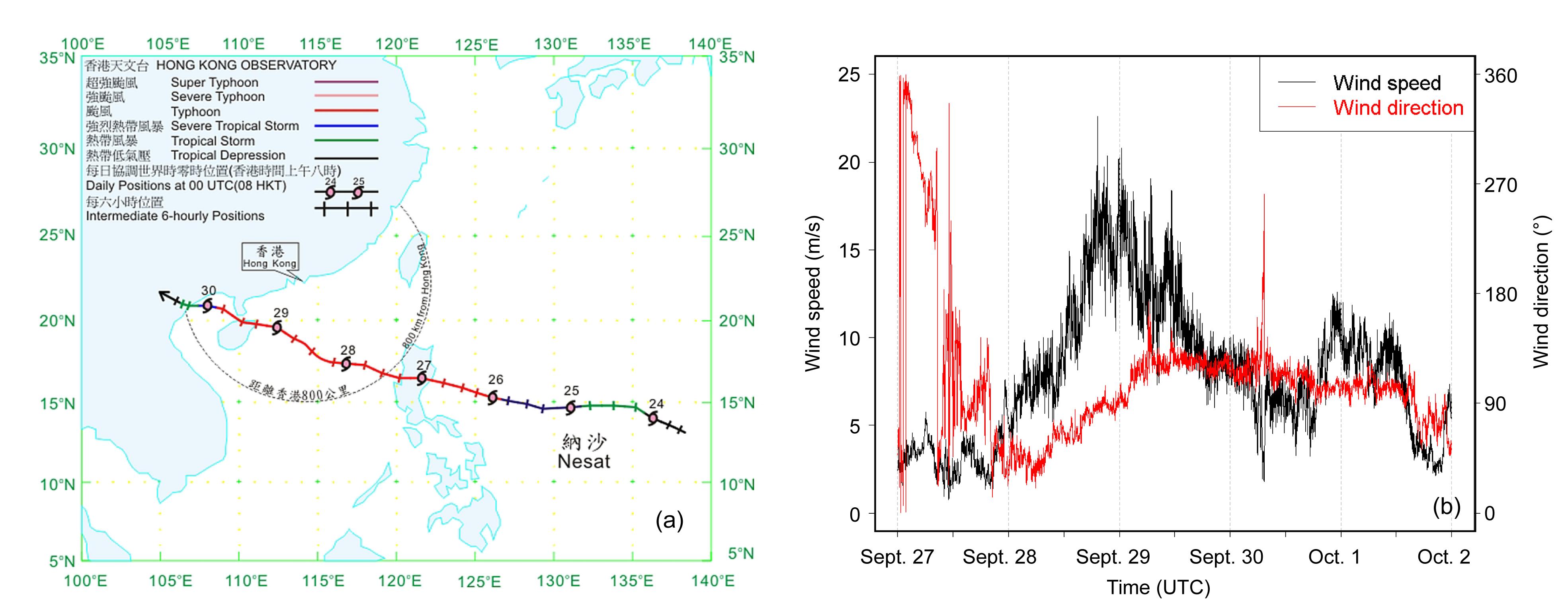
 Typhoon Nesat originated as an area of low pressure over the western North Pacific on Sept. 23, 2011. It moved west-northwest towards Philippines in the next few days and continued to intensify. The track of Nesat is shown in Fig. 2a. The typhoon crossed Luzon, Philippines, on Sept. 27 and entered the South China Sea.




 During the movement of Nesat towards Hainan Island, the winds over the Hong Kong territory gradually picked up. The time series of the surface anemometer reading at the centre of the north runway of HKIA (which is used to represent the winds generally in Hong Kong) is shown in Fig. 2b. It could be seen that, in the period from Sept. 27 to 28, 2011, the winds at the airport picked up gradually from 3 m/s to 8 m/s. The wind direction also changed from north to northeast.

 The winds at the airport reached 22 m/s at about 20 UTC, Sept. 28. They were generally east to southeasterly on that day. The high winds crossing the mountainous terrain of Lantau Island resulted in significant turbulence of orographically-induced nature over the airport region. Nesat continued to track west-northwestwards and made its first landfall over Hainan Island in the afternoon on that day.

 On Sept. 30, Nesat moved further away from Hong Kong. It also made landfall the second time near the China-Vietnam border. Local winds gradually weakened (Fig. 2b).

 An overview of the turbulence intensity in the whole typhoon episode is given in Fig. 3. The time series of the EDR obtained from a number of sources in the period of Sept. 27 to Oct. 2, 2011 are shown, namely, WTWS, LIDAR, TDWR, and flight data. As shown in (Cornman et al., 2008), both the maximum and the median values of the EDR within 3 nautical miles from the runway end are considered, and they are shown in Figs. 3a and 3b, respectively. All the flights in Fig. 3 refer to the aircraft landing at the north runway of HKIA from the west, i.e., runway corridor 07LA.




 In general, various EDR values show similar trends. In terms of height, the LIDAR and aircraft data are similar, namely, about 300 m above sea level at 3 nautical miles to the west of the western threshold of the north runway. At that location, the TDWR’s radar beam is located at about 200 m above sea level. The turbulence intensities calculated from various methods (Fig. 3) reach a maximum in the period between 18 UTC, Sept. 28 and 12 UTC, Sept. 29. On Sept. 30, with the weakening of the local winds, the turbulence intensity also drops gradually. Occasionally there are spikes of rather high EDR values from LIDAR, TDWR, and flight data, e.g., those reaching 0.7 m^2/3·s⁻¹ or above. They have been carefully inspected to be genuine by examining the outputs from the calculation algorithms in the intermediate steps. They are believed to represent the transient nature of mechanical turbulence in terrain-disrupted airflow associated with high winds of a typhoon. Moreover, other effects of the calculation, such as the heights of the beams of the remote sensing meteorological instruments and the choice of the window size in the calculation of EDR, may also contribute to the differences in the EDR values. In particular, for the calculation of LIDAR EDR, a period of several minutes is considered to accumulate a sufficient sample of turbulent eddies. On the other hand, the TDWR EDR is based on individual PPI scans of the radar.

 Comparatively, the EDR time series from WTWS appears to be smoother. In the implementation of EDR estimation in WTWS, the direct EDR values estimated from the surface anemometer readings have been processed through a running 15-min smoothing algorithm (Cheung et al., 2008). As such, WTWS is expected to show the general trend of the turbulence in the study period, which is consistent with the EDR values calculated from other instruments.

7.  Performance of LIDAR EDR

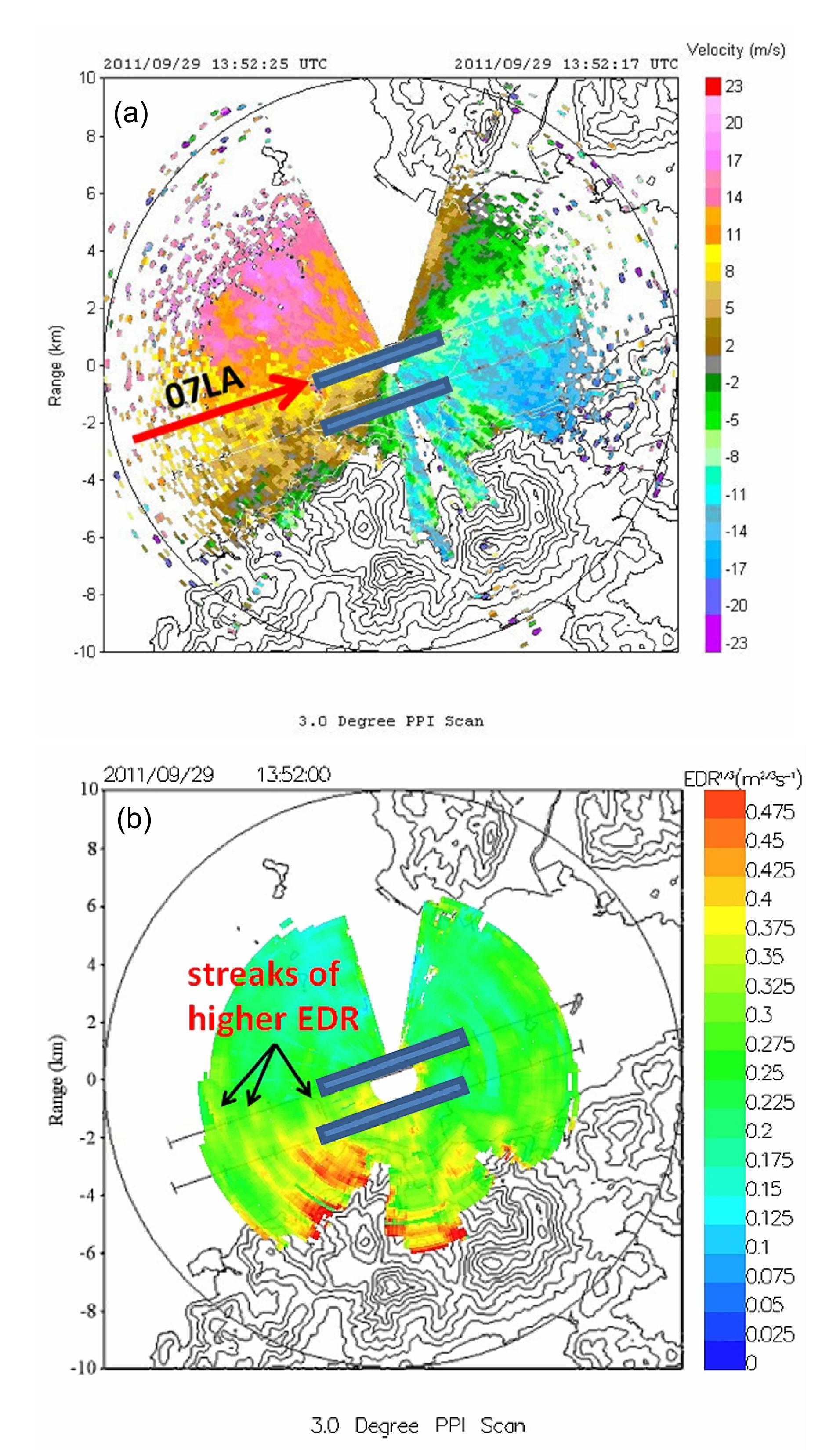
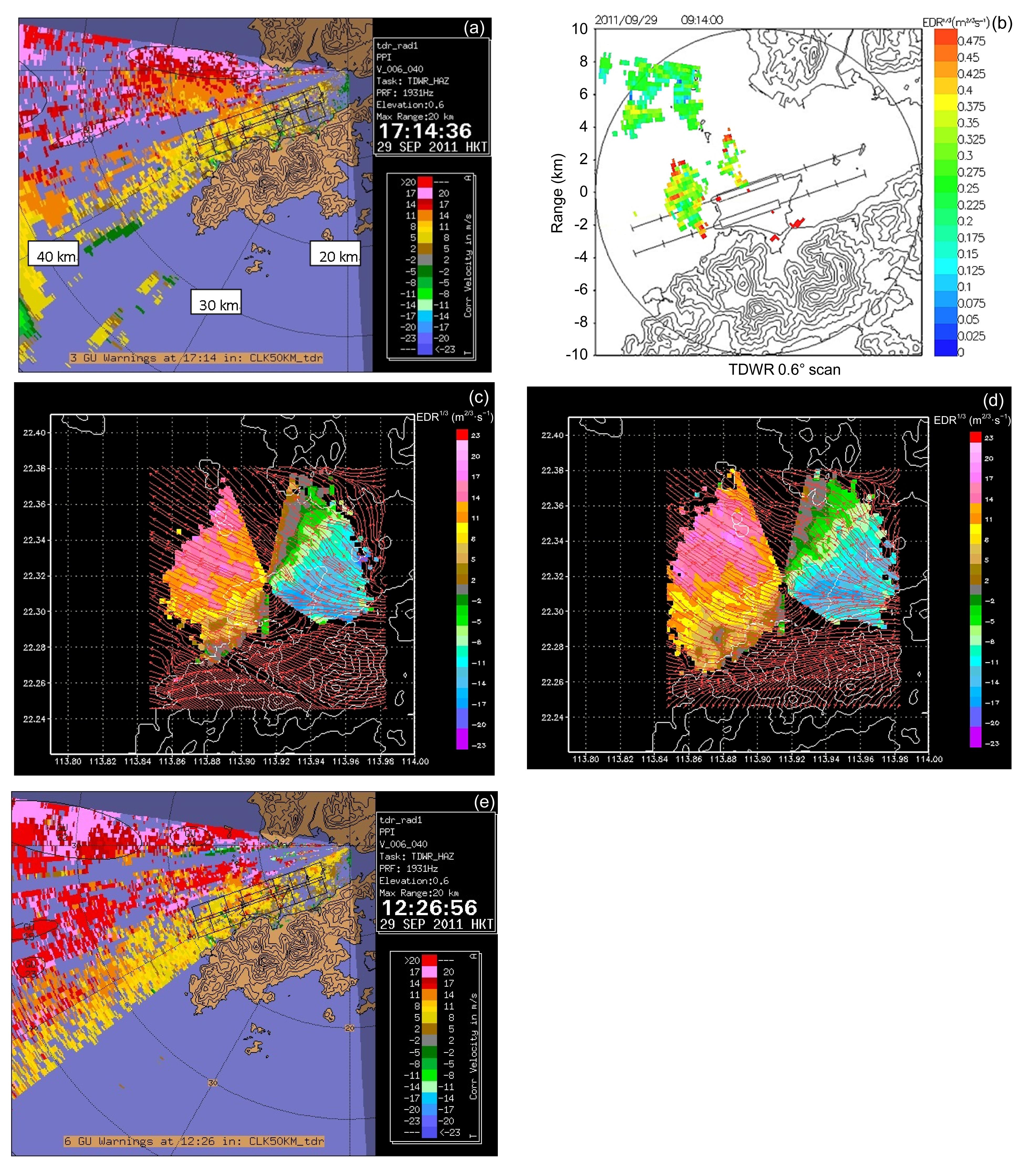
 Before the general performance of LIDAR EDR in the whole typhoon episode is examined, a case study of a typical EDR profile from the LIDAR is presented. The case occurred at 13:52 UTC (21:52 HKT) on Sept. 29, 2011. The radial velocity imagery from the north runway LIDAR in 3° PPI scan is given in Fig. 4a.




 The flow is generally non-uniform in the airport area. In particular, over the sea to the west of HKIA island in which the 07LA runway corridor is located, there are some small blobs of higher wind speed (coloured orange, with a radial velocity of around 11 m/s) with the dimensions of several hundred meters embedded in the prevailing southeasterly flow of about 8 m/s. The corresponding EDR map is shown in Fig. 4b. The turbulence intensity is higher over the sea downstream of the high mountains of Lantau Island, as coloured in yellow to red in Fig. 4b. In particular, there are some short streaks of higher EDR (around 0.4 m^2/3·s⁻¹) affecting the 07LA runway corridor (highlighted in Fig. 4b).

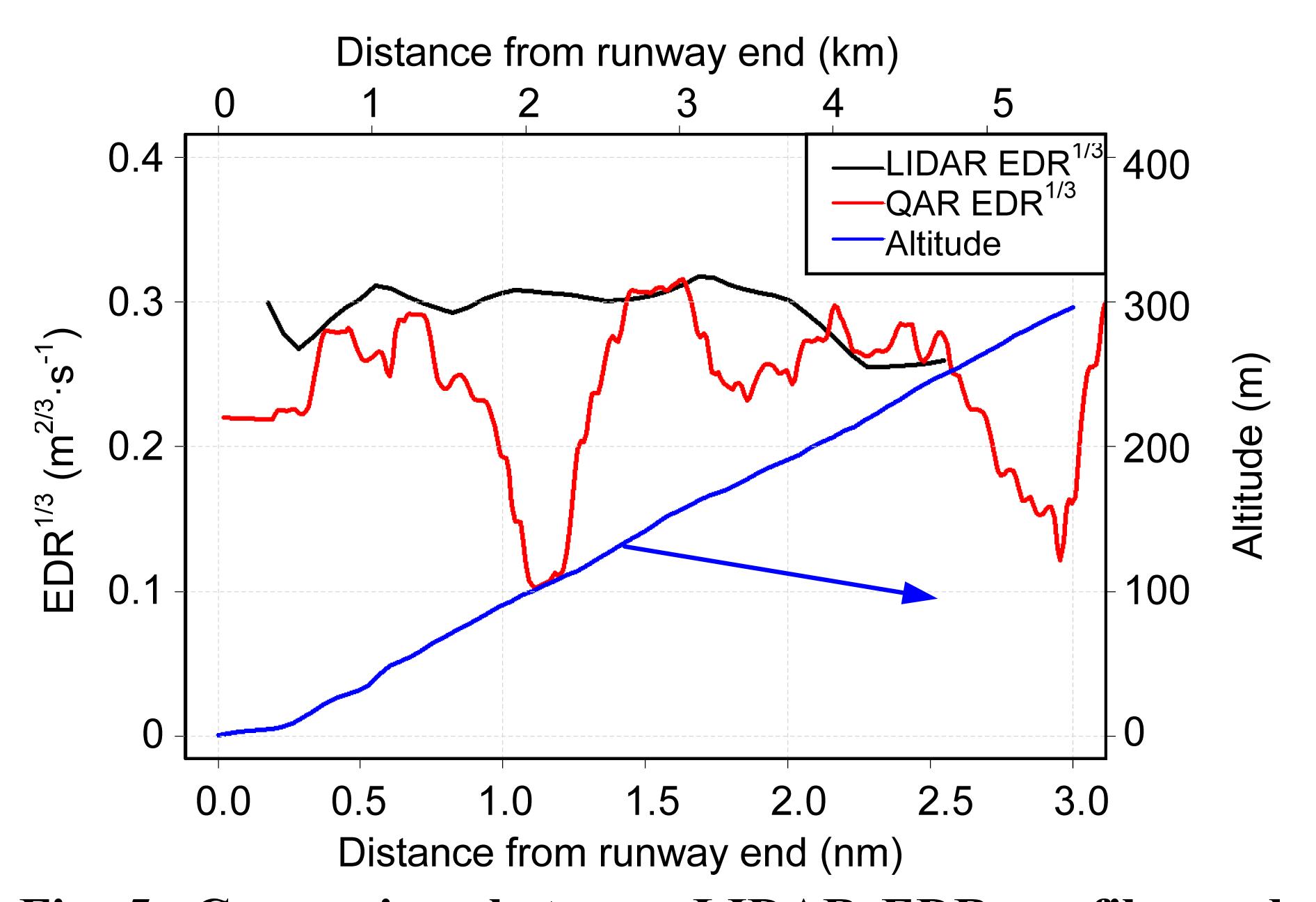
 Flight data are obtained from one aircraft landing at 07LA at the time of Fig. 4. The EDR profiles from LIDAR data and QAR data are shown in Fig. 5. They are found to be generally consistent with each other. One discrepancy is the lower EDR value between 1 and 1.5 nautical miles from the runway end as shown in the flight data, whereas the EDR is rather uniform as calculated the LIDAR over this interval of the runway corridor. This may be expected from various averages adopted in the calculation of LIDAR EDR, namely, consideration of velocity fluctuation over the relatively large area of a subsector (with an areal extent of a couple of kilometers in the direction of the extended runway centerline) and over a certain period of time (15 min).




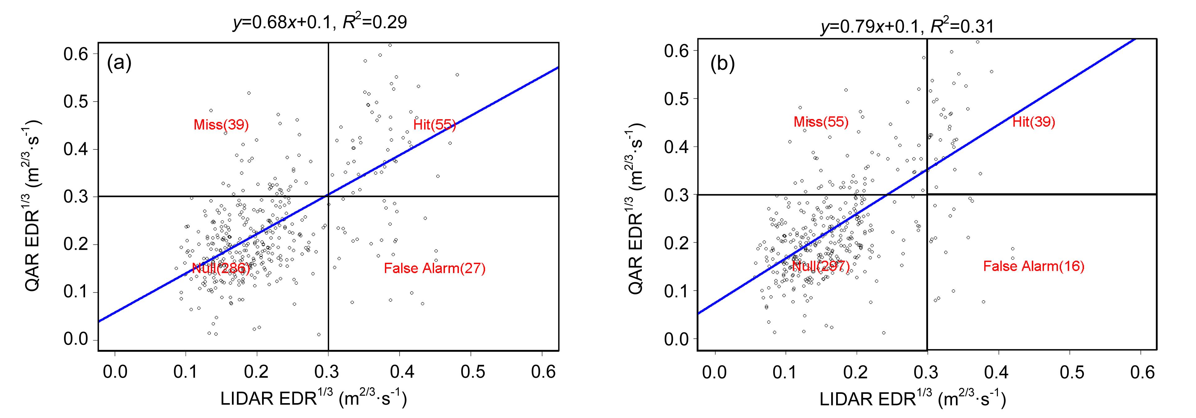
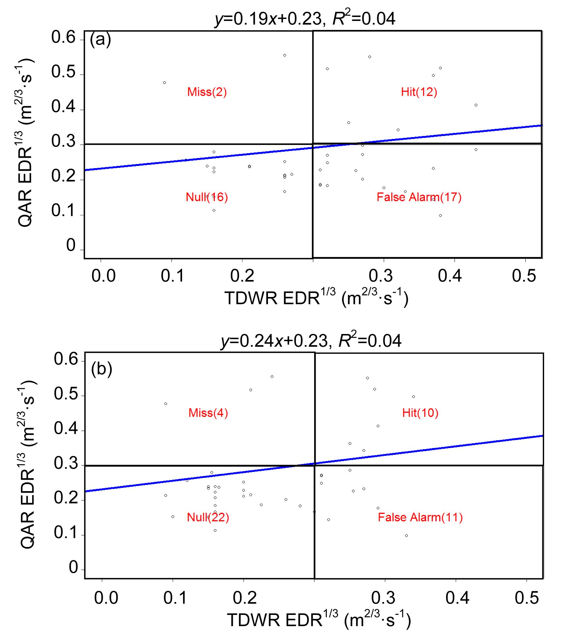
 The maximum and median values of LIDAR EDR and the corresponding EDR from the aircraft are compared in the scatter plots of Figs. 6a and 6b, respectively. The EDR values from the two data sources are correlated with each other to a certain extent, though the correlation coefficients are not very high. This may be expected from the transient nature of turbulence. With the use of the maximum value of EDR for the detection of moderate turbulence within 3 nautical miles from the runway end, the hit rate of flight EDR based on the LIDAR EDR is 58.5% (55/(39+55)), and the false alarm rate is 8.6% (27/(286+27)). With the use of the median value of EDR, the hit rate is 41.5% and the false alarm rate is 5.1%. The majority of the cases are null-null cases, i.e., insignificant turbulence with median or maximum EDR^1/3 value is less than 0.3 m^2/3·s⁻¹.

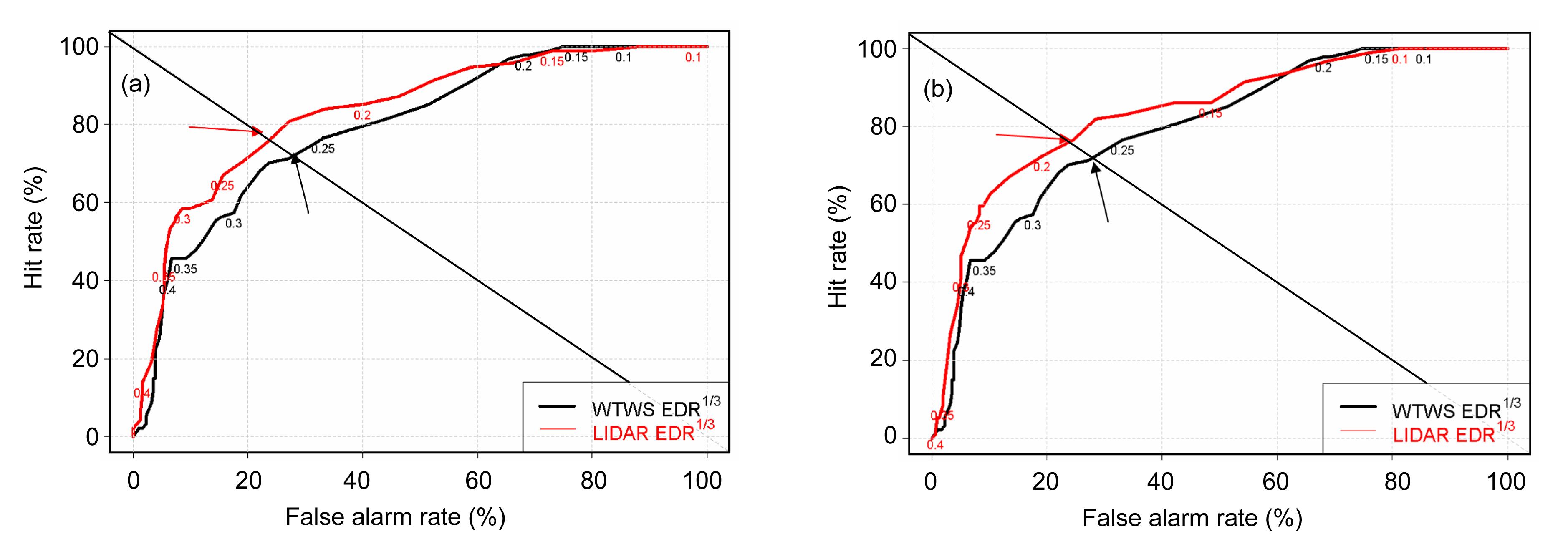
 The threshold of capturing moderate turbulence of the aircraft by LIDAR EDR may be tuned by considering relative operating characteristics (ROC) curve of hit rate versus the false alarm rate. The ROC curve based on the dataset in Fig. 6 is given in Fig. 7, namely, the maximum value in Fig. 7a and median value in Fig. 7b. For the former, a fine-tuned threshold of 0.23 m^2/3·s⁻¹ could be used for the maximum value, resulting in a hit rate of 75.5% (71/(71+23)) and a false alarm rate of 23.3% (73/(73+240)). It is determined by considering the intersection where the ROC curve crosses the diagonal (from upper left to lower right) of the ROC diagram. The fine-tuned value for median value of EDR^1/3 is 0.19 m^2/3·s⁻¹, with similar hit rate (76.6%) and false alarm rate (24.6%). In both cases, the performance of LIDAR EDR is better than that of the WTWS EDR, i.e., the area under the curve is larger for LIDAR than WTWS. Miss events are opposite to hit events, i.e., they could not be captured by the system/equipment under consideration. They are significant to the airport operation, namely, occurrence of significant turbulence as encountered by the aircraft, but could not be alerted in time. For the WTWS EDR, the EDR values are calculated from the anemometer-based regressors and the alerting threshold is adjusted to achieve the best results of low-level turbulence detection by balancing the hit rate and the false alarm rate, similar to that of the LIDAR EDR. The scatter plots of QAR EDR vs. WTWS EDR are similar in appearance to Fig. 6 (not shown), though the individual events falling in each category (hit, miss, false alarm, and null) are different.

8.  Performance of TDWR EDR

 A typical case of EDR values from TDWR during the Typhoon Nesat episode is shown in Fig. 8. It is raining over HKIA and the surrounding area. The radial velocity plot from the lowest PPI scan, namely, 0.6° PPI, is shown in Fig. 8a. The airflow appears to be rather turbulent in the airport region. In particular, over the 07LA runway corridor, there are a couple of blobs with higher wind speed (coloured orange, with a radial velocity of 11 to 14 m/s), each having the dimensions of several hundred meters, embedded in the generally weaker southeasterly flow in the vicinity (coloured yellow, with a radial velocity of 5 to 11 m/s). The corresponding EDR map is shown in Fig. 8b. Over the 07LA runway corridor, the turbulence is generally light to moderate (coloured green, with EDR^1/3 between 0.15 and 0.3 m^2/3·s⁻¹). However, there are isolated spots of stronger turbulence, with EDR^1/3 value reaching 0.375 to 0.45 m^2/3·s⁻¹ (coloured yellow and red).




 The EDR profiles from the TDWR and an aircraft landing at the 07LA at the time of Fig. 8 are shown in Fig. 9a. It could be seen that they are generally consistent with each other. There is an offset of about 0.1 (TDWR EDR relative to QAR EDR), which is related to (1) difference in the location of the TDWR radar beam over the 07LA runway corridor and the location of the aircraft (please refer to the discussion in Section 6 about the heights) and (2) the difference in spatial resolution (aircraft data are essentially point measurements whereas TDWR has a spatial resolution of 150 m). It is noted that this offset is not persistent. For instance, for the cases shown in Figs. 9b and 9c, no systematic offsets could be identified.




 The TDWR EDR and aircraft EDR are compared in Fig. 10. Once again, the results are obtained by considering the whole period of Typhoon Nesat. The correlation between the two datasets does not seem to be good for both the maximum and the median values. Considering moderate turbulence based on the maximum EDR value, the hit rate is 85.7% (12/(2+12)) and the false alarm rate is 51.5% (17/(17+16)).




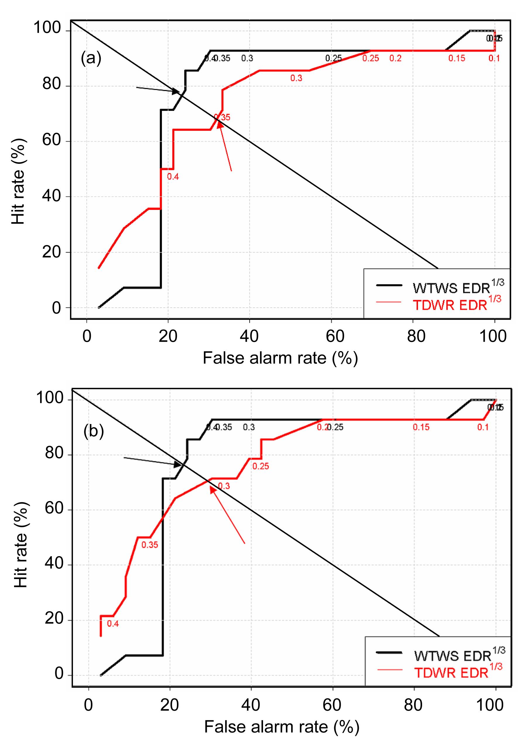
 The performance of the TDWR EDR may be tuned again by considering the ROC curves. The curves for maximum and median values of TDWR EDR are shown in Figs. 11a and 11b, respectively. For the maximum value, the best performing TDWR EDR^1/3 value would be 0.35 m^2/3·s⁻¹, with a hit rate of 71.4% (10/(10+4)) and a false alarm rate of 33.3% (11/(11+22)). The best performing median value would be 0.31 m^2/3·s⁻¹, with a similar hit rate (71.4%) and false alarm rate (30.3%). In general, the performance of TDWR EDR is not so good compared with WTWS EDR, which could be expected from the scatter plots in Fig. 10. Further enhancements of TDWR EDR calculation algorithm are being conducted.




 When both TDWR and LIDAR have good quality data (e.g., not raining extensively), the velocity data from both pieces of equipment could be combined for performing dual-Doppler wind retrieval following the method of Chan and Shao (2007). Some examples of the resulting 2D wind fields can be found in Figs. 8c and 8d. The TDWR image at the time of Fig. 8d is given in Fig. 8e. Such wind field data are useful for the aviation weather forecasters to visualize the wind patterns in the airport area. Please note that there may be some artifacts in the retrieved 2D wind field in the areas without the data from the LIDAR, such as the blind zone of the LIDAR and the sector-blanked area to the south and southeast of the LIDAR.

9.  Combined performance of LIDAR and TDWR EDR

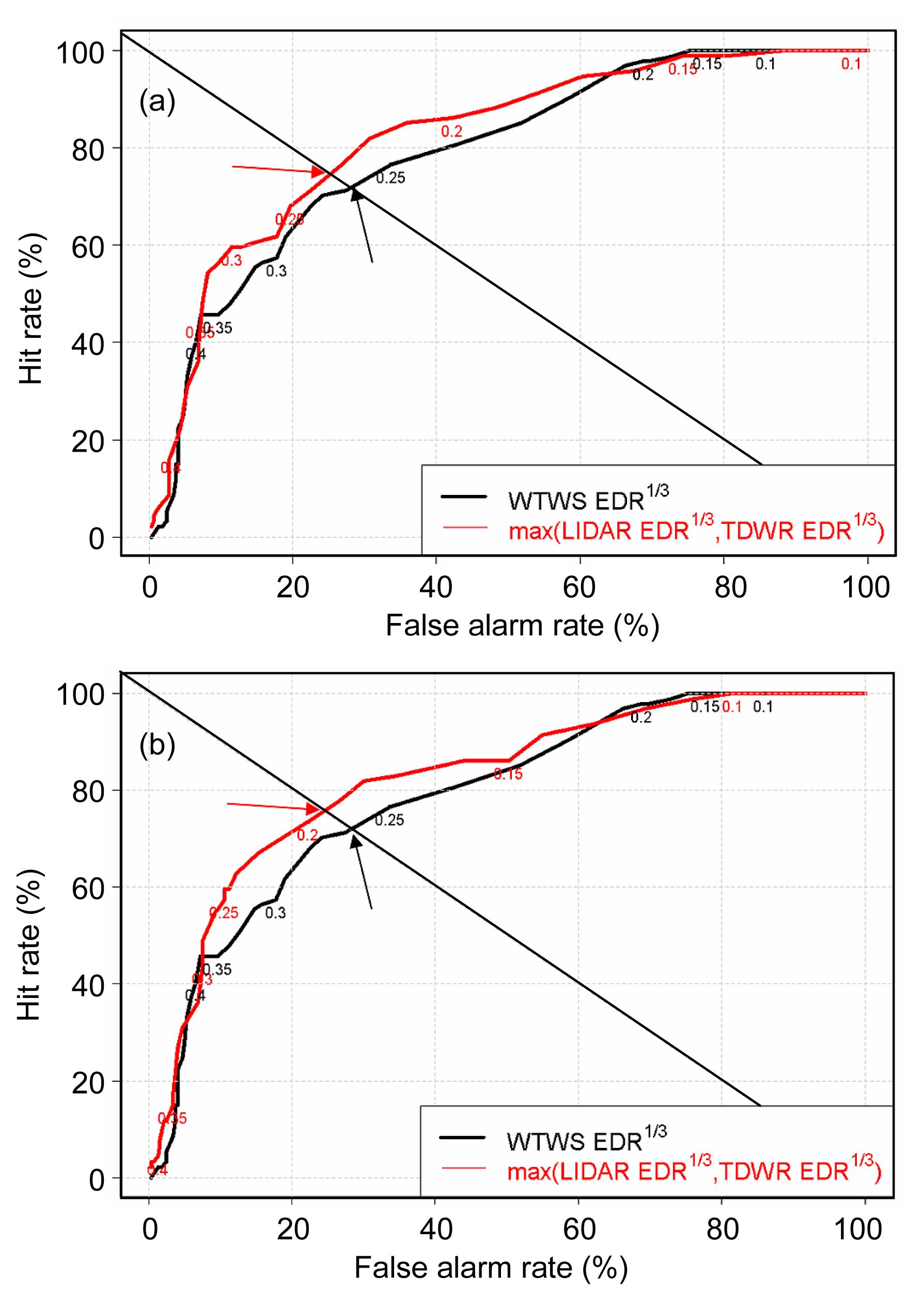
 The EDR values from LIDAR and TDWR are combined in the detection of turbulence by comparing with the flight EDR value, and the performance is studied by comparing with that of WTWS EDR. Two methods are used in combining the LIDAR and TDWR EDRs, namely, the maximum between the maximum LIDAR EDR and the maximum TDWR EDR, and the maximum of the median LIDAR EDR and the median TDWR EDR. They are denoted as “maximum-maximum” and “maximum-median”, respectively.

 The performance of the two kinds of combination values is shown in Fig. 12. The best performing value of “maximum-maximum” is 0.23 m^2/3·s⁻¹ and that of “maximum-median” is 0.19 m^2/3·s⁻¹, which are coincided with those of LIDAR EDR. The combined EDR is slightly better than WTWS EDR, probably due to the larger contribution from the LIDAR EDR. In general, considering the case of Typhoon Nesat, the performance of turbulence detection could be improved over that of WTWS EDR by considering the LIDAR EDR for non-rainy weather conditions. For rainy weather, TDWR EDR still does not perform better than the WTWS EDR, though TDWR is directly measuring the winds and thus turbulence over the runway corridor. Further enhancements of TDWR EDR algorithm would be necessary.

10.  Conclusions

 The performance of LIDAR- and radar-based EDR measurements along the flight paths of HKIA is studied in this paper for a typical case of terrain-induced turbulence in association with cross-mountain airflow of a typhoon. It is examined based on EDR determined from QAR data of the aircraft. EDR measured by these remote sensing meteorological instruments, at least for the LIDAR, performs better than anemometer-based EDR estimate in the existing WTWS algorithm. It is a comprehensive study involving data of hundreds of commercial jets. Moreover, QAR-based EDR measurement is used in the study, which is more objective than the use of the pilot turbulence reports.

 Based on the results of this particular case, it appears that LIDAR-based EDR measurement performs better than WTWS by suitably choosing alerting threshold based on ROC curve. The hit rate reaches 76% and the false alarm rate is just 23%, which could be regarded as having sufficient quality for operational use. The false alarm rate of 23% is considered to be a bit high, but this is the start-of-the-art in the detection of low level turbulence. For instance, in the LIDAR-based windshear alerting system that is in operation at HKIA, the false alarm rate is in the order of 30%, which is still considered to be useful for windshear alerting at the airport. One major challenge in the operational use of LIDAR-based EDR measurement is the rather computationally-demanding calculation process for the structure function approach. Attempts are being made for real-time implementation of this method by parallelizing the calculation algorithm.

 On the other hand, the performance of TDWR-based EDR is not so good in comparison with WTWS-based EDR, even though the radar is making measurements close to the flight paths of the aircraft. Further enhancements to the TDWR-based EDR are being made, for instance, in better handling the windshear term.

 Based on the results of this study, LIDAR-based EDR may be used in non-rainy weather conditions. At times of rain, it would still be preferable to use the WTWS-based EDR. Further study would need to be conducted for other cases of terrain-induced turbulence at HKIA, such as easterly winds in stable atmosphere in spring.

References

[1] Brewster, K.A., Zrnic, D.S., 1986. Comparison of eddy dissipation rate from spatial spectra of Doppler velocities and Doppler spectrum widths. Journal of Atmospheric and Oceanic Technology, 3(3):440-452.
[2] Chan, P.W., 2010. LIDAR-based turbulence intensity calculation using glide-path scans of the Doppler light detection and ranging (lidar) systems at the Hong Kong International Airport and comparison with flight data and a turbulence alerting system. Meteorologische Zeitschrift, 19(6):549-563.
[3] Chan, P.W., Shao, A.M., 2007. Depiction of complex airflow near Hong Kong International Airport using a Doppler LIDAR with a two-dimensional wind retrieval technique. Meteorologische Zeitschrift, 16(5):491-504.
[4] Chan, P.W., Zhang, P., 2012. Aviation Applications of Doppler Radars in the Alerting of Windshear and Turbulence. Doppler Radar Observations-weather Radar, Wind Profiler, Ionospheric Radar, and Other Advanced Applications, InTech,:470
[5] Chan, S.T., Mok, C.W., 2004. Comparison of Doppler LIDAR Observations of Severe Turbulence and Aircraft Data. , 11th Conference on Aviation, Range, and Aerospace Meteorology, American Meteorological Society, Hyannis, MA, USA, :
[6] Cheung, P., Lam, C.C., Chan, P.W., 2008. Estimating Turbulence Intensity along Flight Paths in Terrain-disrupted Airflow Using Anemometer and Wind Profiler Data. , 13th Conference on Mountain Meteorology, Whistler, BC, Canada, :
[7] Cornman, L.B., Meymaris, G., Limber, M., 2008. An Update on the FAA Aviation Weather Research Program’s in situ Turbulence Measurement and Reporting System. , 12th Conference on Aviation, Range and Aerospace Meteorology, American Meteorological Society, Georgia, USA, :
[8] Doviak, R.J., Zrnic, D.S., 2006. Doppler Radar and Weather Observations. Dover Publications Inc.,Mineola, New York :562
[9] Fang, M., Doviak, R.J., Melnikov, V., 2004. Spectrum width measured by the WSR-88D radar: Error sources and statistics of various weather phenomena. Journal of Atmospheric and Oceanic Technology, 21(6):888-904.
[10] Frehlich, R.G., Meillier, Y., Jensen, M.L., Balsley, B., Sharman, R., 2006. Measurements of boundary layer profiles in an urban environment. Journal of Applied Meteorology and Climatology, 45(6):821-837.
[11] Haverdings, H., Chan, P.W., 2010. Quick access recorder (QAR) data analysis software for windshear and turbulence studies. Journal of Aircraft, 47(4):1443-1447.
[12] 2010. Windshear and Turbulence in Hong Kong. Information Booklet for Pilots, :
[13] ICAO (International Civil Aviation Organization), 2010. Meteorological Service for International Air NavigationAnnex 3 to the Convention on International Civil Aviation, ICAO,:206
[14] Labitt, M., 1981. Coordinated Radar and Aircraft Observations of Turbulence. Project Rep. ATC 108, MIT, Lincoln Lab :39
[15] Neilley, P.P., Foote, G.B., Clark, T.L., 1995. Observations of Terrain-induced Flow in the Wake of a Mountainous Island. , 7th Conference on Mountain Meteorology, Breckenridge, CO, 264-269. :264-269.
[16] Shun, C.M., Lau, S.Y., Lee, O.S.M., 2003. Terminal Doppler weather radar observation of atmospheric flow over complex terrain during tropical cyclone passages. Journal of Applied Meteorology, 42(12):1697-1710.
Open peer comments: Debate/Discuss/Question/Opinion