Affiliation(s):
1.
State Key Laboratory of Automotive Simulation and Control, Jilin University, Changchun 130025, China; moreAffiliation(s): 1.
State Key Laboratory of Automotive Simulation and Control, Jilin University, Changchun 130025, China; 2.
Department of Mechanical Engineering, University of California, Berkeley, California 94720, USA; less
Pan Song, Chang-fu Zong, Masayoshi Tomizuka. A terminal sliding mode based torque distribution control for an individual-wheel-drive vehicle[J]. Journal of Zhejiang University Science A, 2014, 15(9): 681-693.
@article{title="A terminal sliding mode based torque distribution control for an individual-wheel-drive vehicle", author="Pan Song, Chang-fu Zong, Masayoshi Tomizuka", journal="Journal of Zhejiang University Science A", volume="15", number="9", pages="681-693", year="2014", publisher="Zhejiang University Press & Springer", doi="10.1631/jzus.A1400101" }
%0 Journal Article %T A terminal sliding mode based torque distribution control for an individual-wheel-drive vehicle %A Pan Song %A Chang-fu Zong %A Masayoshi Tomizuka %J Journal of Zhejiang University SCIENCE A %V 15 %N 9 %P 681-693 %@ 1673-565X %D 2014 %I Zhejiang University Press & Springer %DOI 10.1631/jzus.A1400101
TY - JOUR T1 - A terminal sliding mode based torque distribution control for an individual-wheel-drive vehicle A1 - Pan Song A1 - Chang-fu Zong A1 - Masayoshi Tomizuka J0 - Journal of Zhejiang University Science A VL - 15 IS - 9 SP - 681 EP - 693 %@ 1673-565X Y1 - 2014 PB - Zhejiang University Press & Springer ER - DOI - 10.1631/jzus.A1400101
Abstract: This paper presents a torque distribution method for an individual-wheel drive vehicle, in which each wheel is controlled individually by its own electric motor. The terminal sliding mode technique is employed for the motion control so as to track the desired vehicle motion obtained by interpreting the driver’s commands. Thus, finite-time convergence of the system’s dynamic errors can be achieved on the terminal sliding manifolds, as compared to the well-used linear sliding surface. By considering nonlinear constraints of the tire adhesive limits, a simple yet effective distribution strategy is introduced to allocate the motion control efforts to each of the four wheels. Through the use of a high-fidelity CarSim full-vehicle model, vehicle stability and handling performance of the proposed controller is evaluated in both open- and closed-loop simulations.
Darkslateblue:Affiliate; Royal Blue:Author; Turquoise:Article
Article Content
1. Introduction
With the rapid development of electric motors and electronic communications, there is a trend in the automotive industry towards the use of electrified propulsion systems together with electronic control systems to achieve fuel efficiency and to improve handling performance. Almost all automakers throughout the world have been studying and promoting electric vehicles (EVs) for energy and environmental considerations. Individual-wheel drive (IWD) is a promising technique for EVs in which all wheels are controlled independently by their own in-wheel/hub motors (Hori, 2004).
Because of the inherent characteristics of electric motors in which the torque can be negative, it is necessary for the global chassis control (GCC) system to coordinate the individual traction and braking actions of the four wheels. There are two main tasks in the GCC system (Johansen and Fossen, 2013). The first one is to compute a vector of virtual inputs to be applied to the vehicle so as to meet the motion control objectives of a given application. The other is to allocate these efforts to the individual actuators such that the total forces and moments generated by all actuators amount to the motion control efforts. In the design of the motion controller, the nonlinearity of the vehicle dynamics is usually handled by employing the sliding mode control (SMC) method (Mokhiamar and Abe, 2004; Li et al., 2008; Wang and Longoria, 2009). A terminal sliding mode control (TSMC) is a type of sliding control, in which the finite-time convergence and quick responsiveness can be achieved on the terminal sliding manifold (Liu and Wang, 2012). It has been successfully applied to applications of vehicle longitudinal (Kim et al., 2007) and lateral (Ren et al., 2011) control, but no study has been previously made regarding its effects on the combined motion control. In the matter of control allocation, different optimization methods have been proposed (Mokhiamar and Abe, 2004; Ono et al., 2006; Li et al., 2008; Wang and Longoria, 2009; Chen and Wang, 2011), although none of them are computationally efficient. An alternative plan is to employ the pseudo-inverse method to map the relationship between the motion control efforts and the actuator efforts (Weiskircher and Müller, 2012), but this does not consider the actuator saturation and consequently has limited practical utility.
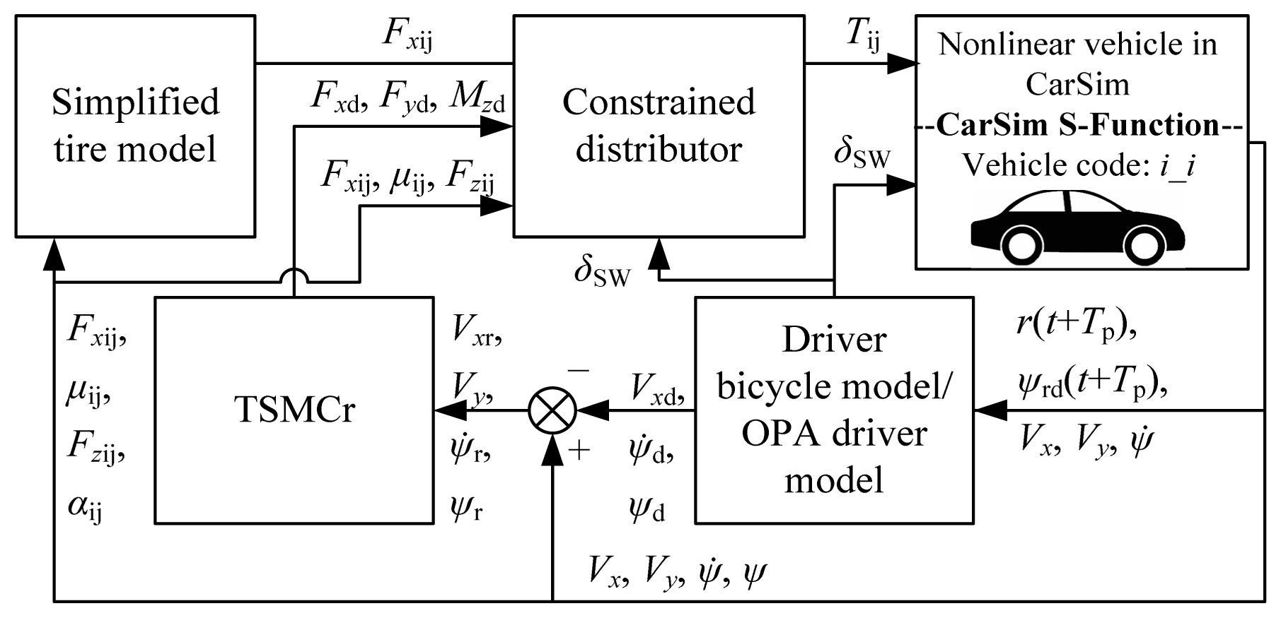
In this paper, a novel torque distribution controller is developed for an IWD EV (Fig. 1). First, the bicycle model and the optimal preview acceleration (OPA) driver model is used to provide the steering wheel angles δSW in the open- and closed-loop maneuvers to compute the desired vehicle states Vxd, , and ψd. Second, a terminal sliding mode controller (TSMCr) is designed to generate the motion control efforts, i.e., Fxd, Fyd, and Mzd, to track the desired motion commands, in which the steady-state tracking errors can be eliminated in finite time. Third, while the longitudinal tire forces of the IWD vehicles can be controlled individually, for the trade-off between computational precision and real-time performance, this paper employs a simplified tire model to effectively calculate lateral tire forces with acceptable accuracy. Thus, nonlinear constraints of the tire adhesive limits can be determined accordingly. Last, by considering these constraints, a distributor effectively allocates the motion control efforts to each of the four wheels based on a novel strategy, which divides the task into several unconstrained distributions. It should be noted that for concerns of cost, maintenance and safety, no four wheel steering (4WS) or active front steering (AFS) system is involved and the only controlled variables are the four wheels’ traction/braking torques.
Fig.1 Structure of proposed torque distribution controller The explanations of the variables are given in Section 2.1 as well as in Section 3
2. System modeling
2.1. Vehicle dynamics model
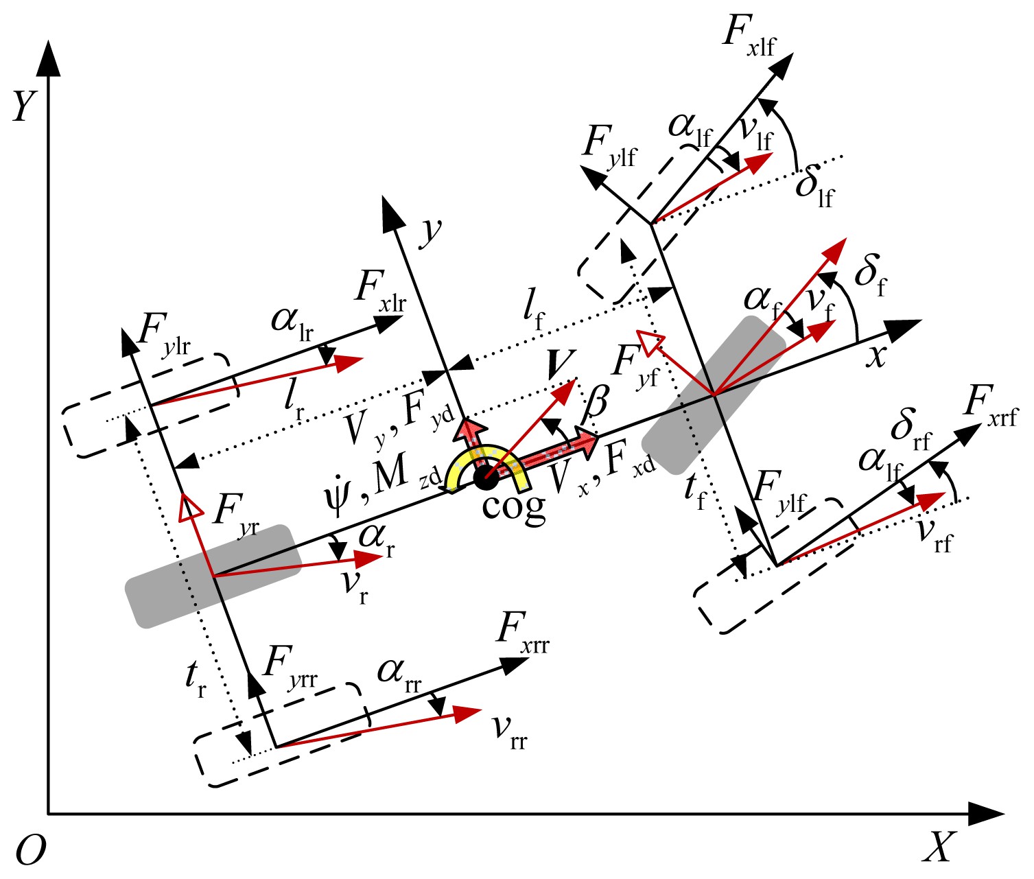
For the model-based controller design, the vehicle is modeled as a 3-DOF (three degrees of freedom) double track model. Its coordinate system is shown in Fig. 2. ,
,
where Vx and Vy are the longitudinal and lateral velocities of the vehicle at cog (center of gravity), respectively; ψ is the yaw angle, the first- and second-order time derivatives of which are the yaw rate and yaw angular acceleration, respectively; CD is the drag coefficient factor; Af is the vehicle front area; ρ is the air density; m is the vehicle mass; Iz is the moment of inertia around the vertical axis; the motion control efforts Fxd, Fyd, and Mzd are the desired longitudinal force, lateral force, and yaw moment, respectively; Fxij is the tire longitudinal force, which is controlled timely (due to the fast response of the electric motor) and precisely (via an accurate measurement of the motor torque); Fyij is the tire lateral force, which can be calculated by a tire model; the first subscript of (·)ij denotes the left (l) or right (r) side of the vehicle, and the second denotes the front (f) or rear (r) axle. The corresponding matrices are ,
,
where lf and lr are the distances from cog to front and rear axles, respectively; tf and tr are the front and rear wheel treads, respectively; δlf and δrf are respectively the steering angles of the left-front and right-front wheels, where the Ackerman steering principle is applied, expressed as follows: ,
where the minus (plus) sign is for the left (right) wheel; L is the wheelbase of the vehicle, L=lf+lr; δf is the front wheel steering angle.
Fig.2 Schematic of vehicle model
A simple yet powerful tool to describe the vehicle lateral dynamics is the well-known bicycle model, as shown in Fig. 2. The matrix form of this model is expressed as Eq. (6), in which the left and right side wheels are combined to one wheel, and the lateral tire forces Fyf and Fyr are proportional to the tire sideslip angles αf and αr, respectively. ,
where Cαf and Cαr are the tire cornering stiffnesses of the front and rear axles, respectively.
The relationship between the vehicle sideslip angle β and the lateral velocity can be expressed as .
2.2. Wheel model
With the use of electric motors to drive all the wheels, an IWD EV can control the longitudinal tire forces individually based on the following equation: ,
where Tij is the traction/braking torque exerted by the electric motor; Tbij is the friction torque of the braking system and is assumed to be known; Jij is the wheel spin inertia; is the wheel spin acceleration; Rij is the wheel effective rolling radius; fij is the rolling resistance coefficient; Fzij is the tire vertical load, which can be expressed as follows:
where the minus (plus) sign is for the left (right) tire; g is the gravitational constant (9.8 m/s2); ms is the sprung mass of the vehicle; kf and kr are the lateral weight-shift distribution ratios on the front and rear axles, respectively; hs is the sprung mass height; ax and ay are the longitudinal and lateral accelerations at cog, respectively, and are given by
2.3. Tire model
A simple tire model proposed by Sakai et al. (2002) is used to depict the relationship between the lateral force and the sideslip angle in the tire stable and monotonic region. By using the arctangent function to fit the experimental curve, the tire model can be formulated as follows:
where μ is the tire-road friction coefficient; Cα is the tire cornering stiffness; α is the tire sideslip angle, which is obtained by Eq. (12). Here, the value of the fitting constant i is changed to ‘2.9’ to improve the fitting accuracy at relatively large sideslip angles.
where σij is the angle between the velocity of wheel center and the longitudinal axle of the vehicle body. They are given by
where the minus (plus) sign is for the left (right) wheel.
3. Driver-vehicle system
3.1. Reference model
This study assumes that the driver’s task is only to keep the vehicle tracking at given speed profiles. So the desired longitudinal velocity is independent from the steering task:
where Vxd is the desired longitudinal velocity of the vehicle at cog; Vxr is the longitudinal velocity error; Vx0 is the initial longitudinal velocity of the vehicle at cog; axd is the driver acceleration or deceleration command.
For stability consideration, the undesired vehicle sideslip motion that generates Vy should be suppressed to the minimum level, which can be effectively controlled by systems such as 4WS and AFS. However, these complex systems increase the overall cost and require additional maintenance. Moreover, since the vehicle’s lateral dynamics are greatly influenced by the active intervention of the AFS system, non-cooperative behaviors may occur between the human driver and the AFS system when they hold different targets (Na and Cole, 2013). This can cause an inexperienced driver to get stressed and increase his/her risk of a serious road accident. Therefore, we study the IWD EV with a conventional front-wheel-steering configuration and use a torque distribution approach to control the vehicle’s motion.
The steady-state yaw rate response of the bicycle model in Eq. (6), i.e., steady-state yaw rate gain, , is obtained by
where Ks is defined as the understeer gradient, which usually has a negative value. It can be determined that the understeer gradient is actually a time-varying coefficient with the tire cornering stiffness varying at different vertical loads, road conditions, and slip ratios. Also, a non-zero Ks makes
a nonlinear function of Vx. Furthermore, the driver tends to maneuver the vehicle according to its linear response, so that hereafter the value of Ks is set to be ‘0’, which implies that the steady-state yaw rate gain is Vx/L.
3.2. Driver model
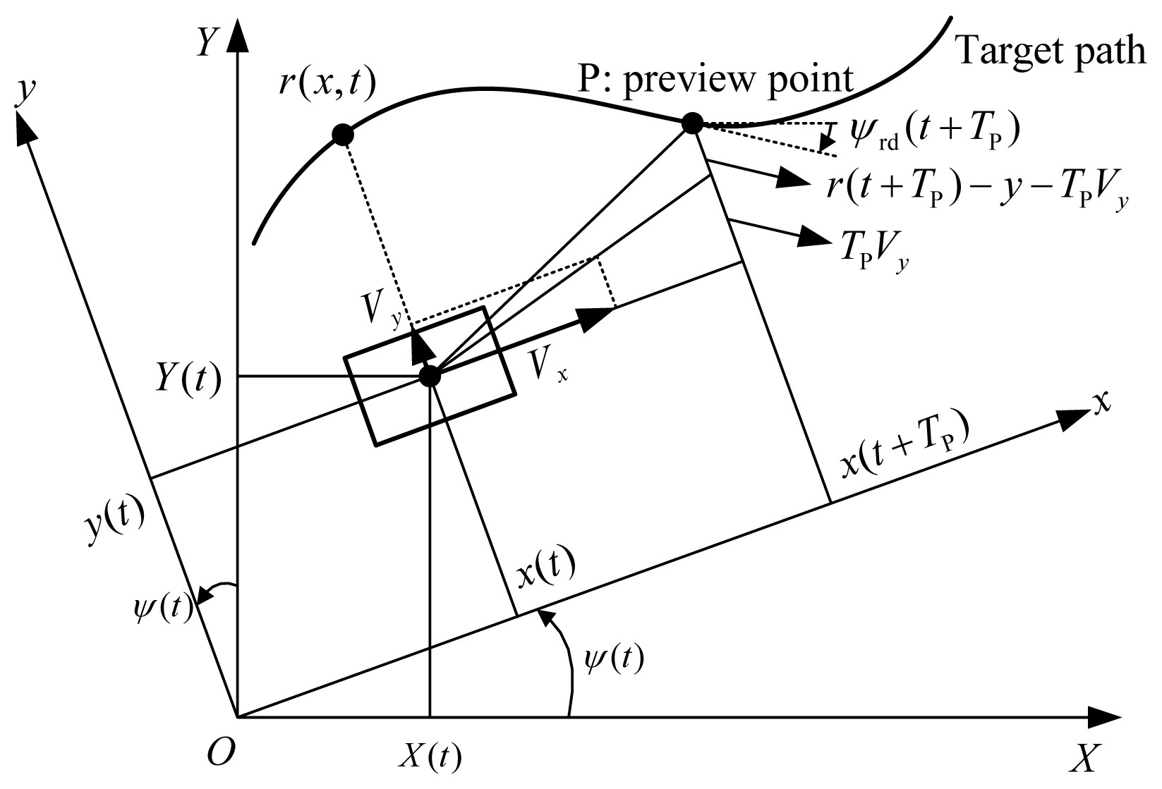
The experiments should contain the open-loop maneuvers in order to verify the tracking performance of the proposed controller. Nevertheless, the controller should also be tested in the closed-loop maneuvers, so that the driver’s reactions to the vehicle dynamic responses can be studied and analyzed. This study employs the OPA driver model to mimic the human driver behavior (Guo and Guan, 1993). By using the schematic representation of Fig. 3 and assuming the vehicle proceeds with the current longitudinal and lateral velocities, the previewed lateral error between the desired path and the actual vehicle position ε is defined by ,
where Tp is the preview time; r(t+Tp) is the desired path after Tp; y is the lateral offset of vehicle at cog.
Fig.3 Schematic of OPA driver model geometry
Fig. 4 shows the block diagram of this single-point preview model, which exerts the steering input in order to provide the optimal lateral acceleration and to minimize the previewed lateral error. Eq. (17) indicates that the OPA driver model predicts the vehicle’s future position based on the dynamic response of the aforementioned bicycle model.
where Gay is the steady-state steering gain, which reflects the yaw dynamics of the internal model anticipated by the driver and is proportional to the aforementioned steady-state yaw rate gain; is the optimal front wheel steering angle. The driver’s actual input to the vehicle is the steering wheel angle δSW, given by ,
where iSW is the steering system ratio; TC is the driver correction time; TN is the driver action delay; TD is the driver brain response delay; and s is the Laplace operator.
Fig.4 Block diagram of OPA driver model
For the lane-keeping task, the driver exerts steering effort not only to eliminate the deviation error, but also to minimize the orientation error with respect to the road. Moreover, it was discovered that accumulation of the yaw rate tracking error could cause the undesired vehicle yaw angle which greatly affects the vehicle heading and path-following accuracy (Wang and Longoria, 2009). Thus, a yaw angle control effort is considered to mitigate this effect. To sum up, the yaw error ψr and the yaw rate error are given by
where ψrd is the road path heading angle after TP, as shown in Fig. 3.
4. Terminal sliding mode control (TSMC)
The global fast TSMC proposed by Park and Tsuji (1999) is employed to design the sliding surfaces s1 and s2, while the nonsingular TSMC technique proposed by Feng et al. (2002) is applied to design the sliding surface s3. The sliding surfaces are defined by ,
,
,
where αieq and βieq are the strictly positive constants of TSMC (i=1, 2, 3); pi and qi are the positive odd numbers and pi>qi. In particular, for i=3, we also have: 1<p3/q3<2.
Because the longitudinal and lateral velocities follow the dynamics of the first-order system in Eq. (1), the control laws u1 and u2 are directly derived from the sliding surfaces by letting s1 and s2 be equal to ‘0’, expressed as Eq. (23). Meanwhile, the yaw motion follows the dynamics of a second-order system, thus the control law is obtained from the differential equation, given by Eq. (24).
where u3n is the approaching law for the sliding surface s3. Here, the nonlinear reaching law u3n proposed by Ren et al. (2011) rather than a linear one is adopted to achieve the finite-time convergence of and when , and thus allows us to have a better control performance. ,
where α3n and β3n are strictly positive constants; p3n and q3n are positive odd numbers and p3n>q3n.
To sum up, the control laws are given by ,
,
.
The global fast sliding surface for the controllers u1 and u2 is expressed as Eq. (29), of which the convergence time is ts when the initial state x(0)≠0 reaches x=0 which is given by Eq. (30). .
By analyzing the solutions of the differential equation, expressed as Eq. (31), the finite-time convergence for the nonsingular TSMCr u3 occurs from the initial state s3(0)≠0 to s3=0. .
Hence, we have .
Then it is straightforward to determine that the yaw angle error ψr will reach ‘0’ along the sliding mode in finite time (Liu and Wang, 2012).
For stability analysis, the Lyapunov functions are selected as
Then we have: ,
,
.
Then the sliding conditions are satisfied and the sliding surfaces are attractive. Note that if the desired forces and moment cannot be generated due to the friction circle limitations of the four wheels, the stability of the proposed TSMCrs cannot be guaranteed. The friction circle of each tire would directly affect the range of the control efforts. The inequality constraint of the motion control efforts is written as ,
where Wr is a constant weight balancing forces/moment, which is chosen as the reciprocal of the typical length between cog and road wheels (Ono et al., 2006). When the control efforts are calculated to be greater than this constraint, the motion control efforts would be limited by a ratio of τu. Note that this loose bound is to ensure that the desired motions are theoretically realizable before the efforts are distributed to the actuators, a precise limitation of the bound will be developed and handled in the torque distribution strategy, which will be illustrated in the next subsection.
5. Constrained torque distribution
The motion control efforts produced by TSMCr need to be distributed to the electric motors driving the four wheels. The functional relationship between the motion control efforts and the controlled variables can be compactly written as Eq. (38), which serves as a redundant linear constraint for the torque distribution problem.
where B is a 3×4 matrix representing the effectiveness of the actuators. There are 3 motion control objectives but only 4 controlled variables, which has limited potential for an optimal distribution. Furthermore, optimization approaches usually require large computational efforts and are not suitable for real-time applications. Thus, assuming that the pseudo-inverse B+ exists, this study distributes the control efforts by calculating the torques with uact=B+Fud. The tire adhesive limit should also be considered as an additional constraint, which can be described by the friction ellipse concept ,
where the values of the coefficients Cxij and Cyij are set to ‘1’ due to the use of the simple tire model in Eq. (11), which defines the friction limitation as a circle rather than an ellipse. However, it is still difficult and time-consuming to distribute torques directly under these nonlinear constraints of four tires.
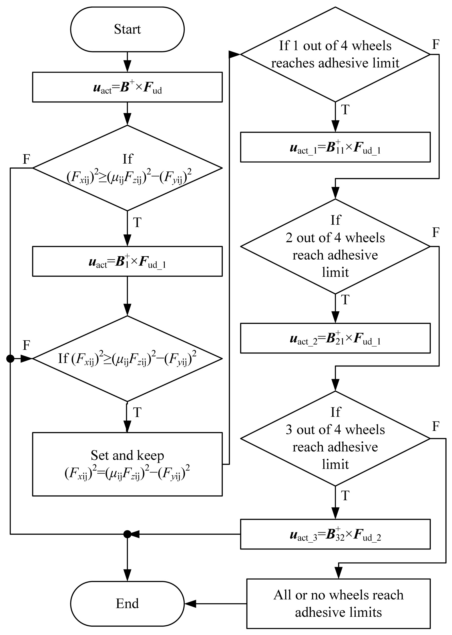
This study presents an efficient way to divide this problem into no more than 5 unconstrained distributions (Fig. 5). Note that for small lateral accelerations, all the 3 control efforts desired by TSMCr can be achieved; when Fyd is large, this force should be ignored, where the sideslip motion is suppressed mainly by the driver’s steering effort rather than by the controller itself; when 3 out of 4 wheels reach their adhesive limits, Fxd is also ignored and only Mzd is left to be achieved, which is thought to be more critical to the vehicle’s handling stability.
Fig.5 Tire force distribution strategy
Here, for notation simplification, uact_i and Fud_j can be expressed as Eqs. (40) and (41), respectively; Bij is the corresponding matrices of uact_i and Fud_j. Particularly, B1 is the corresponding matrix of uact and Fud_1. The superscript (∙)+ denotes the pseudo-inverse operator.
Once the tire longitudinal forces are obtained, the traction/braking torque of each wheel is calculated by Eq. (7).
6. Results and discussion
The proposed torque distribution method is designed in the MATLAB/Simulink environment. As depicted in Fig. 1, an A-Class Hatchback full-car model built in CarSim is employed here for the controller validation. Some of the vehicle’s parameters are listed in Table 1. Three simulation cases including both open- and closed-loop maneuvers are conducted. The responses of the vehicles with TSMCr and the traditional sliding mode controller (SMCr) proposed by Wang et al. (2009) are compared with each other. The unconstrained distribution approaches are also added for comparison, which does not take into consideration the tire adhesive limits.
Table 1
Parameters of the vehicle model
Parameter
Value
Total mass of vehicle, m (kg)
830
Sprung mass of vehicle, ms (kg)
747
Moment of inertia around vertical axis, Iz (kg·m2)
1157.1
Sprung mass height, hs (m)
0.54
Longitudinal distance of cog to front axle, lf (m)
1.103
Longitudinal distance of cog to rear axle, lr (m)
1.244
Front wheel tread, tf (m)
1.416
Rear wheel tread, tr (m)
1.375
Steering system ratio, isw
16.4
6.1. Open-loop step-steer maneuver
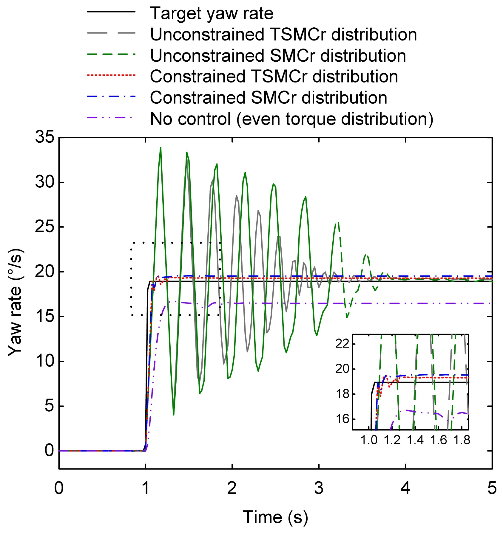
In the open-loop simulation, the driver model is not involved, and the yaw error ψr is thus neglected. The vehicle is subjected to a step-like steering input at 1.0 s, with a front steering angle δf=2° (δSW=32.8°). The speed remains constant at 80 km/h and the road friction coefficient is 0.85. The vehicle dynamic responses are shown in Figs. 6 and 7 and Table 2.
Fig.6 Yaw rate responses in step steer maneuver
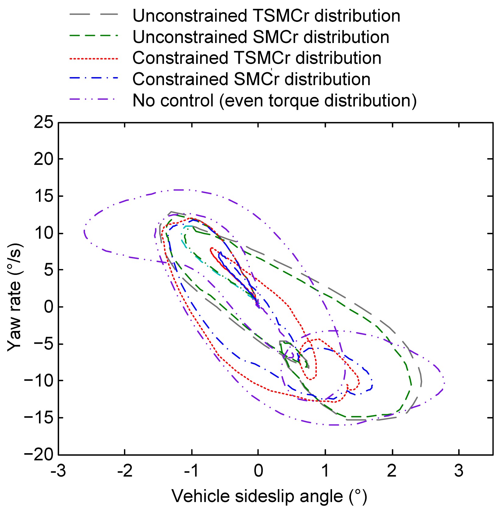
Fig.7 Vehicle sideslip angle responses in step steer maneuver
Table 2
RMS of yaw rate error and sideslip angle
Vehicle configuration
Yaw rate error, (°/s)
Sideslip angle, β (°)
Unconstrained TSMCr
4.1839
18.8986
Unconstrained SMCr
5.2888
23.4745
Constrained TSMCr
1.0641
1.0788
Constrained SMCr
1.1395
1.1161
No control
3.0111
0.5633
From Fig. 6, it can be seen that since the target yaw rate represents the neutral steering response, the conventional IWD vehicle without control tends to understeer and is not able to reach the yaw rate desired by the driver. For the vehicles using the unconstrained distribution methods, as soon as the steering commands are applied, their states oscillate in the time domain but can still be stabilized to the target values. This can be explained by the fact that in the high speed cornering case with a relatively large steering angle, the tire forces distributed by the unconstrained distribution method are beyond the tire adhesive limits, such that one or more tires are saturated and they cannot provide enough forces within the tire adhesive limits which can amount to the total yaw moment required by the motion controller. This problem can be effectively solved by the proposed constrained distribution strategy. Both vehicles with the constrained methods can accurately respond to the desired yaw rate, Table 2 shows that the constrained TSMCr provides the best control performance with the minimum error.
As shown in Fig. 7, the suppression of the vehicle sideslip angles by these distribution methods is restricted due to the limited impacts on the lateral motion by the longitudinal tire forces, thus each controller acts more like a joint system of cruise control (CC) and direct yaw control (DYC), which controls the longitudinal and yaw motions simultaneously. However, the vehicles with the unconstrained methods lose their stabilities, while the constrained ones can still control the vehicle sideslip motion to be stable, whereas their sideslip angles are slightly larger than that of the conventional vehicle. The root mean square (RMS) values of the sideslip angles can be found in Table 2. Note that the counter steering effect of the conventional vehicle is eliminated by the proposed method, which does not produce the reversed sideslip angle and has a faster lateral response than without control.
6.2. Closed-loop maneuver
To further evaluate the control effects, closed-loop simulations are conducted and performed as the handling tests, in which the OPA model provides the driver’s steering inputs for the lane-keeping tasks. Note that the road path heading angle ψrd used to calculate the yaw error ψr in Eq. (19) is obtained by some road information acquisition algorithm, which is not presented in this study.
6.2.1. Double-lane-change
The first closed-loop simulation is a double-lane-change (DLC) maneuver, with a constant longitudinal velocity of 100 km/h and a road friction coefficient of 0.5. The results are shown in Figs. 8 to 10.
Fig.8 Vehicle trajectories in a DLC maneuver
Fig.9 Driver-vehicle system responses in a DLC maneuver
Fig.10 Driver steering angles in a DLC maneuver
It is shown in Fig. 8 that in the attempt to control the conventional vehicle to track the given path accurately, the OPA driver model cannot provide the appropriate steering effort due to the mismatch between the characteristics of the neutral steer anticipated by the driver and the handling response of the vehicle without control, and this therefore causes large lateral deviations from the ideal path. However, vehicles with both the unconstrained approaches do not lose lateral stability as they do in the step-steer maneuver and show fairly good path-following performance. Despite that, the constrained approaches provide good path-tracking performance. This is primarily because the constrained distribution methods can generate the motion control efforts determined respectively by TSMCr and SMCr as much as possible (especially when the vehicles are cornering with large lateral acceleration) within the tire adhesive limits. The RMS value of the lateral offset of the constrained TSMCr is 0.1693 m, compared to that of the constrained SMCr which is 0.2023 m.
Fig. 9 shows the driver-vehicle system responses depicted in the phase plane, where the controller with the tighter trajectory but higher value of yaw rate response is supposed to maximize the stability margin and the vehicle responsiveness. It can be attributed to the aforementioned mismatch effect that the trajectory of the response of the vehicle without control appears much looser. Its maximum yaw rate and sideslip angle as well as those of the vehicles with unconstrained methods are located in the fourth quadrant of the plot, which indicates these vehicles tend to be less stable and perform poorly before entering into the second straight section of the DLC path. At the same time, the vehicle without control needs extra steering effort to be stabilized and is difficult for the driver to manipulate, as shown in Fig. 10. Both the constrained distribution methods attain good control performance, whereas the constrained TSMCr gives better handling performance (the tightest trajectory in Fig. 9) and increases maneuverability (the least steering effort in Fig. 10).
6.2.2. Hard braking through a μ-split surface
The second closed-loop simulation is the μ-split braking, which is mainly for the longitudinal dynamics validation. As shown in Fig. 11, the road is divided along a straight line with two different surfaces with μ=0.8 on the left side and μ=0.2 on the right side. The driver attempts to decelerate the vehicle from 120 km/h to 0 as quickly as possible and also steers the vehicle in order to stay in this straight lane.
Fig.11 Vehicle trajectories in μ-split maneuver (laterally-stable ABS vs. common ABS)
During the simulation testing, it was discovered that neither the two unconstrained methods nor the even torque distribution could stabilize the vehicle in this type of maneuver. Hence, the common and the laterally-stable anti-lock brake systems (ABS) are employed here to compare their control effects with each other (Mitschke and Wallentowitz, 1972). Figs. 11 and 12 show the results. It can be seen that although the maximum lateral offset of the laterally-stable ABS is only 0.0027 m, compared to that of the common one, which is 15.4727 m, it still takes 14.2 s for the former to stop the vehicle at 229.7168 m, more than twice as much braking time and distance as those of the common ABS. This is because, to avoid the additional yaw-moment when braking the vehicle, the laterally-stable ABS makes the longitudinal tire forces on both sides be equal to the lesser of the right side, and thus decreases its braking performance. For the common ABS, the vehicle drifts towards the μ-high side of the road, which causes shorter braking distance and time, meanwhile its maximum lateral velocity reaches up to 80 km/h. It can be concluded that both methods fail to balance the trade-off between the lateral stability and the braking efficiency.
Fig.12 Velocities in μ-split maneuver (laterally-stable ABS vs. common ABS)
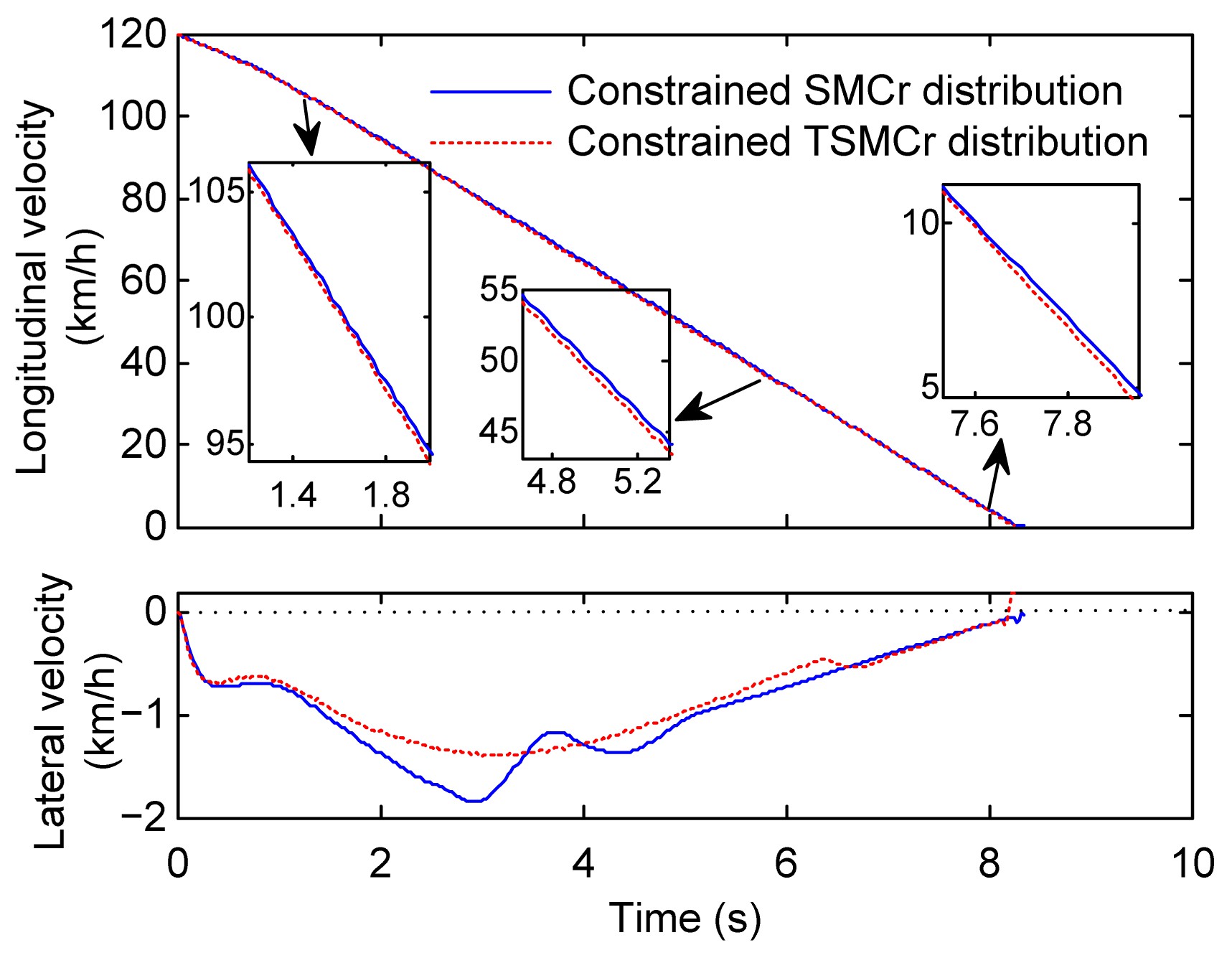
The constrained methods with TSMCr and SMCr are validated in Figs. 13 to 15. Fig. 13 shows that the proposed distribution strategy can fully utilize the road adhesion capability and both controllers provide vehicles with good braking efficiency (the vehicle with TSMCr stops in 8.25 s at 142.0866 m and the one with SMCr stops in 8.35 s at 142.7459 m) by not losing lateral stability (the maximum lateral offsets of TSMCr and SMCr are 0.5049 m and 0.6074 m, respectively) while the latter yields a slightly worse performance. The reason can be explained that with the same initial conditions the state errors of longitudinal and lateral velocities of the TSMCr converge to 0 more rapidly than those of the SMCr do, as shown in Fig. 14. Therefore, the vehicle with TSMCr has a shorter braking time with less lateral deviations which hence results in a shorter braking distance. Fig. 15 also suggests that due to its faster convergence of the yaw rate error, TSMCr offers a better tracking performance than SMCr.
Fig.13 Vehicle trajectories in μ-split maneuver
Fig.14 Velocities in μ-split maneuver
Fig.15 Yaw rate responses in μ-split maneuver
7. Conclusions
In this paper, a novel torque distribution approach for an IWD vehicle is introduced in the design of the TSMC based controller to adjust and coordinate the torques from four electric motors. The proposed controller alters the handling characteristics of the vehicle from understeering to neutral steering so that the driver can manipulate the vehicle more easily without having his/her steering effort compensated for nonlinearities in vehicle yaw response. It also operates as a speed controller, which can accurately execute the driver’s acceleration and deceleration commands without degrading steering performance. Although no active steering system is used here, lateral stability is guaranteed and the sideslip motion is, to some extent, suppressed by the controller. Additionally, the constrained distribution methods deal with nonlinear constraints of the tire adhesive limit efficiently and effectively.
Simulation results indicate that due to its fast and finite time convergence, and high steady-state precision, TSMCr provides more improved control effects than SMCr does. Moreover, the constrained distribution approach also significantly improves vehicle stability and handling performance. On an overall evaluation, the constrained TSMC based controller meets the design requirements and shows the best performance among all schemes during our study.
Note that an IWD vehicle is a highly redundant system, which is more inclined to take the risk of actuator failure. Integrating fault tolerant control into this chassis control system will be performed in future work.
[1] Chen, Y., Wang, J., 2011. Energy-efficient control allocation with applications on planar motion control of electric ground vehicles. , American Control Conference, 2719-2724. :2719-2724.
[2] Feng, Y., Yu, X., Man, Z., 2002. Non-singular terminal sliding mode control of rigid manipulators. Automatica, 38(12):2159-2167.
[3] Guo, K., Guan, H., 1993. Modelling of driver/vehicle directional control system. Vehicle System Dynamics, 22(3-4):141-184.
[4] Hori, Y., 2004. Future vehicle driven by electricity and control-research on four-wheel-motored “UOT Electric March II”. IEEE Transactions on Industrial Electronics, 51(5):954-962.
[5] Johansen, T.A., Fossen, T.I., 2013. Control allocation—A survey. Automatica, 49(5):1087-1103.
[6] Kim, D.J., Park, K.H., Bien, Z., 2007. Hierarchical longitudinal controller for rear-end collision avoidance. IEEE Transactions on Industrial Electronics, 54(2):805-817.
[7] Li, D., Du, S., Yu, F., 2008. Integrated vehicle chassis control based on direct yaw moment, active steering and active stabiliser. Vehicle System Dynamics, 46(S1):341-351.
[8] Liu, J., Wang, X., 2012. Advanced Sliding Mode Control for Mechanical Systems, Springer,:
[9] Mitschke, M., Wallentowitz, H., 1972. Dynamik der kraftfahrzeuge. Springer,Berlin :
[10] Mokhiamar, O., Abe, M., 2004. Simultaneous optimal distribution of lateral and longitudinal tire forces for the model following control. Journal of Dynamic Systems, Measurement, and Control, 126(4):753-763.
[11] Na, X., Cole, D.J., 2013. Linear quadratic game and non-cooperative predictive methods for potential application to modelling driver–AFS interactive steering control. Vehicle System Dynamics, 51(2):165-198.
[12] Ono, E., Hattori, Y., Muragishi, Y., 2006. Vehicle dynamics integrated control for four-wheel-distributed steering and four-wheel-distributed traction/braking systems. Vehicle System Dynamics, 44(2):139-151.
[13] Park, K.B., Tsuji, T., 1999. Terminal sliding mode control of second-order nonlinear uncertain systems. International Journal of Robust and Nonlinear Control, 9(11):769-780.
[14] Ren, D., Zhang, J., Zhang, J., 2011. Trajectory planning and yaw rate tracking control for lane changing of intelligent vehicle on curved road. Science China Technological Sciences, 54(3):630-642.
[15] Sakai, S.I., Sado, H., Hori, Y., 2002. Dynamic driving/braking force distribution in electric vehicles with independently driven four wheels. Electrical Engineering in Japan, 138(1):79-89.
[16] Wang, J., Longoria, R.G., 2009. Coordinated and reconfigurable vehicle dynamics control. IEEE Transactions on Control Systems Technology, 17(3):723-732.
[17] Weiskircher, T., Mller, S., 2012. Control performance of a road vehicle with four independent single-wheel electric motors and steer-by-wire system. Vehicle System Dynamics, 50(sup1):53-69.
Open peer comments: Debate/Discuss/Question/Opinion


Open peer comments: Debate/Discuss/Question/Opinion
<1>