Similar articles

Abstract: Short pitch rail corrugations were observed on a recently opened Chinese high-speed line. On the basis of field measurements and observations of corrugations occurred on the high-speed line, a 3D transient rolling contact model is developed using the explicit finite element (FE) method to investigate high-speed vehicle-track interactions in the presence of rail corrugations. The rotational and translational movements of the wheel are introduced as initial conditions in the model. The frictional rolling contact between the wheel and the corrugated rail is solved by a penalty method based surface-to-surface contact algorithm with Coulomb’s law of friction. The contact filter effect is considered automatically by the finite size of the contact patch. Through specifying a time-dependent driving torque applied to the wheel axle, the tangential vehicle-track interaction on the corrugated rail is analyzed in the time domain together with the normal one at different traction levels and at rolling speeds of up to 500 km/h. This analysis focuses on detailed contact solutions, such as distributions of the pressure, surface shear stress, Von Mises (V-M) stress, and frictional work. The corrugation dimensions, traction level, and rolling speed are varied to investigate their influences, building a solid basis for further studying the material damage mechanisms. A theory is proposed based on the simulations to explain the observed phenomenon that the corrugation gradually stabilizes. The traditional multi-body approach is found to overestimate the dynamic wheel-rail interaction on a corrugated rail.

钢轨波磨处高速轮轨滚动接触行为与波磨发展的模拟研究

为求解钢轨（短波）波磨处的高速轮轨瞬态滚动接触建立有限元模型，研究影响高速钢轨波磨发展的重要因素。 1. 求解不同牵引条件下轮轨间的瞬态法和切向滚动接触问题，并考虑真实轮轨几何和钢轨波磨，最高模拟速度达500 km/h；2. 基于模拟结果，解释了中国高速线路上发现的钢轨波磨很快稳定下来的现象。 1. 详细分析钢轨波磨处高速轮轨瞬态滚动接触的法、切向解以及由此导致的V-M等效应力和摩擦功沿轨面的波动；2. 变化波磨波长、波深及重要滚动参数如速度和牵引系数等，研究它们对波磨处滚动接触行为的影响；3. 对比上述有限元模型与传统多体动力模型在波磨处的法向轮轨力结果。 1. 法、切向轮轨力及法、切向接触应力均随着波磨几何呈周期性波动，但相位略有差异，V-M等效应力和摩擦功的波动形式接近切向接触应力；2. 牵引系数越大，波磨处V-M等效应力和摩擦功的波动范围越大；3. 名义参数下，对于所研究高铁系统，波长为80 mm左右、速度为250-300 km/h时波磨的动态响应最大，这与现场观测相符；4. 传统多体动力模型会高估钢轨波磨激励的法向轮轨力；5. 钢轨波磨会逐渐稳定下来，通过速度越高进入稳定越快。
高速钢轨波磨；轮轨滚动接触；车辆-轨道耦合动力学；牵引系数；显式有限元法

1.  Introduction

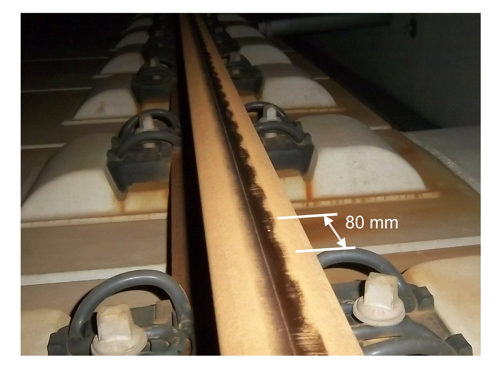
 Rail corrugation is a long-standing problem observed worldwide on many kinds of railway tracks, including tram, metro, traditional railway, heavy haul, and high-speed tracks. Once present, corrugation can worsen the wheel-rail and vehicle-track interactions, leading to poor ride quality and an exacerbated rate of deterioration of the system, e.g., rail support failure (Zhou and Shen, 2013). Recently, rail corrugation, particularly short pitch rail corrugation (hereinafter referred to as corrugation for short), was observed on a recently opened high-speed line in China, causing great concern in the industry. Fig. 1 shows a corrugated rail section on the high-speed line.




 It is well known that corrugation should be a consequence of the accumulation of irregular wear and/or irregular plastic deformation (i.e., the material damage mechanism). Such irregular material damage is likely to be caused by certain eigen-modes of the vehicle-track system excited by some imperfections in the system (i.e., the wavelength fixing mechanism), and the unstable wheel-rail rolling contact resulting from those eigen-modes is the immediate cause. Considering different material damage and wavelength fixing mechanisms, Grassie and Kalousek (1993) and Grassie (2005) classified corrugation into six different categories based on engineering experience, which significantly increased the understanding of corrugation.

 The corrugation mechanisms proposed by Grassie and Kalousek (1993), Grassie (2005), and Knothe and Groβ-Thebing (2008) imply that the key to understanding and predicting corrugation initiation and development is to solve the dynamic vehicle-track interaction and the transient wheel-rail rolling contact. The present work employs a 3D transient rolling contact finite element (FE) model to solve the high-speed wheel-rail rolling contact and the vehicle-track interaction on a corrugated rail in the time domain. This FE model is valid for a rolling speed of up to 500 km/h. A Chinese high-speed railway system is considered. Emphasis of analysis is placed on detailed contact solutions. On the basis of numerical results and field measurements, a better understanding of the mechanism of corrugation development is achieved.

 Traditionally, the vehicle-track interaction on corrugation sites was treated without detailed wheel-rail contact modeling. A simplified Hertz spring was usually employed to represent the contact, together with beams for rails and lumped masses for wheels, respectively (Knothe and Grassie, 1993; Hiensch et al., 2002; Wu and Thompson, 2004; Knothe and Groβ-thebing, 2008; Nielsen, 2008; Xie and Iwnicki, 2008; Iwnicki et al., 2009; Li et al., 2009; Xiao et al., 2010; Zhai et al., 2013). Moreover, most traditional models considered only the normal wheel-rail interaction (Knothe and Grassie, 1993; Hiensch et al., 2002; Wu and Thompson, 2004; Nielsen, 2008; Xie and Iwnicki, 2008; Iwnicki et al., 2009; Li et al., 2009). Nevertheless, the importance of the tangential interaction can be seen from the fact that both the plastic deformation and wear of rails are dominated by the tangential contact load on many corrugation sites, such as on corrugated curves. Taking into account the tangential interaction, Clark et al. (1988) proposed a mechanism of slip-stick vibrations to explain the occurrence of corrugation. Knothe and Groβ-Thebing (2008) and Groβ-Thebing et al. (1992) treated the tangential interaction by using a viscous damper to simulate the steady rolling contact, and the combination of a viscous damper and a spring for the non-steady case. Kalker (1990)’s creep coefficient was employed to determine the characteristics of the viscous damper for the steady rolling contact, and a frequency-dependent creep coefficient (Gross-Thebing, 1989) for the corresponding parameters of the non-steady case. In addition, approaches have also been developed (Iwnicki et al., 2009) to derive the dynamic tangential contact force from the normal contact force and the geometric and material properties of the wheel and rail (Afshari and Shabana, 2010).

 Recent studies have shown that the structural flexibility of the wheelset has a significant influence on the vehicle-track interaction (Ripke and Knothe, 1995; Chaar and Berg, 2006), and even the rotation of the wheel might also play an important role in high frequency vehicle-track dynamics under certain conditions (Baeza et al., 2008). Wen et al. (2005), Pang and Dhanasekar (2006), and Pletz et al. (2009) considered the detailed geometries of the wheel and rail to take their flexibility into account, but only the normal wheel-rail interaction was solved for cases at joints or in crossings.

 The FE modeling approach employed in this study origins from that published in (Li et al., 2008). This approach has been validated by Li et al. (2008; 2011) and Molodova et al. (2011) for the high frequency vehicle-track interaction at squats (in the frequency range between a few hundred and about 2000 Hz), and by Zhao and Li (2011) for the normal and tangential contact solutions. Li et al. (2012) employed the FE modeling approach to study the wheel-rail rolling contact on corrugation and the resulting wear pattern at a speed of 108 km/h, for which a ballasted track was considered. However, the transient rolling contact of a wheel over a corrugated rail at high speeds has not been studied yet.

 Following the same modeling approach, a 3D transient rolling contact FE model is developed for a slab track system of the Chinese high-speed line shown in Fig. 1 to study the corrugation phenomenon. The main advance of the model is that a rolling speed of up to 500 km/h can be simulated, while the maximum rolling speed considered in previous studies was 140 km/h on a ballasted track. In the model, the actual geometries of a wheelset and a rail are included by a mesh of solid elements, based on which a detailed surface-to-surface contact algorithm is employed to solve the transient rolling contact in the time domain. The flexibility of the vehicle and track subsystems and the wheel-rail continua are both included, and the rolling-sliding behavior of the wheel on the rail is simulated. The contact filter effect, which eliminates the corrugation components with a wavelength close to or less than the width of the contact patch (Knothe and Groβ-Thebing, 2008), is considered inherently. Hence, transient contact stresses, including both normal and tangential stresses, and their derivatives are obtained through the numerical simulation, together with the resultant contact forces. These ensure the applicability of the FE model to high-frequency vehicle-track interaction on corrugation sites. Furthermore, idealized corrugation models are applied and simulated to better understand the fundamentals of the corrugation phenomenon, even though measured corrugation profiles can be introduced. For clarity and ease of explanation, the case of a smooth rail (without any irregularities) is analyzed before considering corrugations.

2.  Model descriptions

2.1.  FE model

2.1.1.  An overview

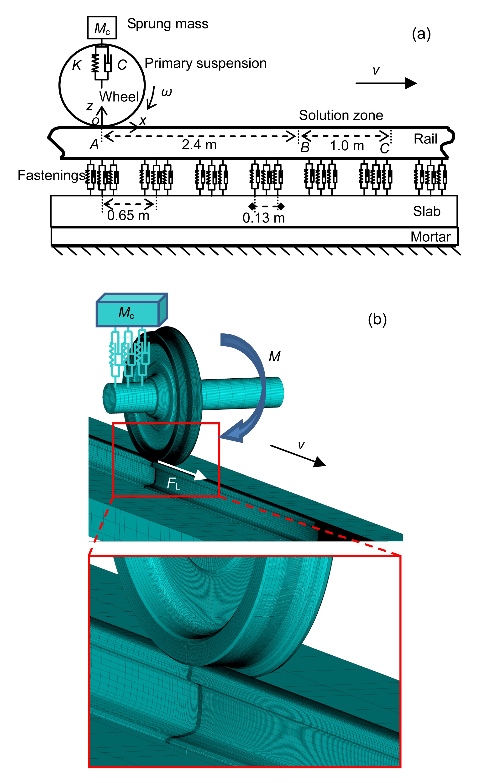
 Fig. 2 illustrates a 3D transient rolling contact FE model developed with ANSYS/LS-DYNA, which considers a high-speed vehicle and a typical slab track on a Chinese high-speed line. The modeling approach for the vehicle is the same as that used by Li et al. (2008) and Zhao and Li (2011). The track is composed of the rail, fastenings, slabs, and the mortar layer. For the investigated high-speed line, the minimum radius of curvature is 7000 m, on which the lateral movement of the wheelset is very well controlled, as predicted by multi-body simulations performed in the State Key Laboratory of Traction Power in Southwest Jiaotong University, China. Further considering that the rolled distance of the wheelset in a typical simulation in this study is less than 3.5 m, the lateral movement of the wheelset becomes negligible. Therefore, only a half wheelset and a half straight track are modeled in view of the symmetry of the system (Fig. 2b), and the lateral movement of the wheelset and the track are ignored. The simulated track is 15.2 m long and includes 24 fastenings.




 A Lagrangian mesh of solid elements is applied to the wheelset and the rail. The minimum element size is 1.1 mm, used in the contact surface of the solution zone (BC in Fig. 2a), where irregularities such as corrugation are applied by modifying the coordinates of the nodes involved. The wheel profile is of the type LM_A and the rail is the standard CN60 with an inclination of 1:40. A penalty method based surface-to-surface contact algorithm is employed to solve the wheel-rail rolling contact, in which Coulomb’s law of friction is used. A mesh of solid elements is also applied to the slabs and the mortar layer. A fastening system is simulated by 12 groups of parallel springs and dampers (three columns in the longitudinal and four rows in the lateral direction). In total, there are 1.46×10⁶ elements and 1.29×10⁶ nodes.

 For solution, boundary conditions are applied as follows: symmetric boundary conditions are applied to the axle ends of the wheelset and to the rail ends; the bottom of the mortar layer is fixed; the fastenings, the slabs, and the mortar layer can only move vertically. Table 1 lists the values of the parameters involved. To simulate the worst case scenario, the sprung mass M _c is determined by considering the weight of the loaded coach, the non-uniform distribution of the weight on different wheels, and the dynamic loads at low frequencies. A 3D right-handed Cartesian coordinate system (Oxyz) is defined, of which the origin O is located in the initial position of the contact patch center (position A in Fig. 2a, hereinafter referred to as the initial position of the wheel). The x axis is defined along the rolling direction (i.e., the longitudinal direction), and the z axis is in the vertical direction. Note that the difference between the vertical direction and the normal direction of the contact is negligible in this study since no lateral movement of the wheelset is considered. Such an FE model, developed specially for investigations into high frequency dynamics, is not suitable for low frequency vibrations such as vehicle hunting.

2.1.2.  A typical process of numerical simulation and the explicit time integration

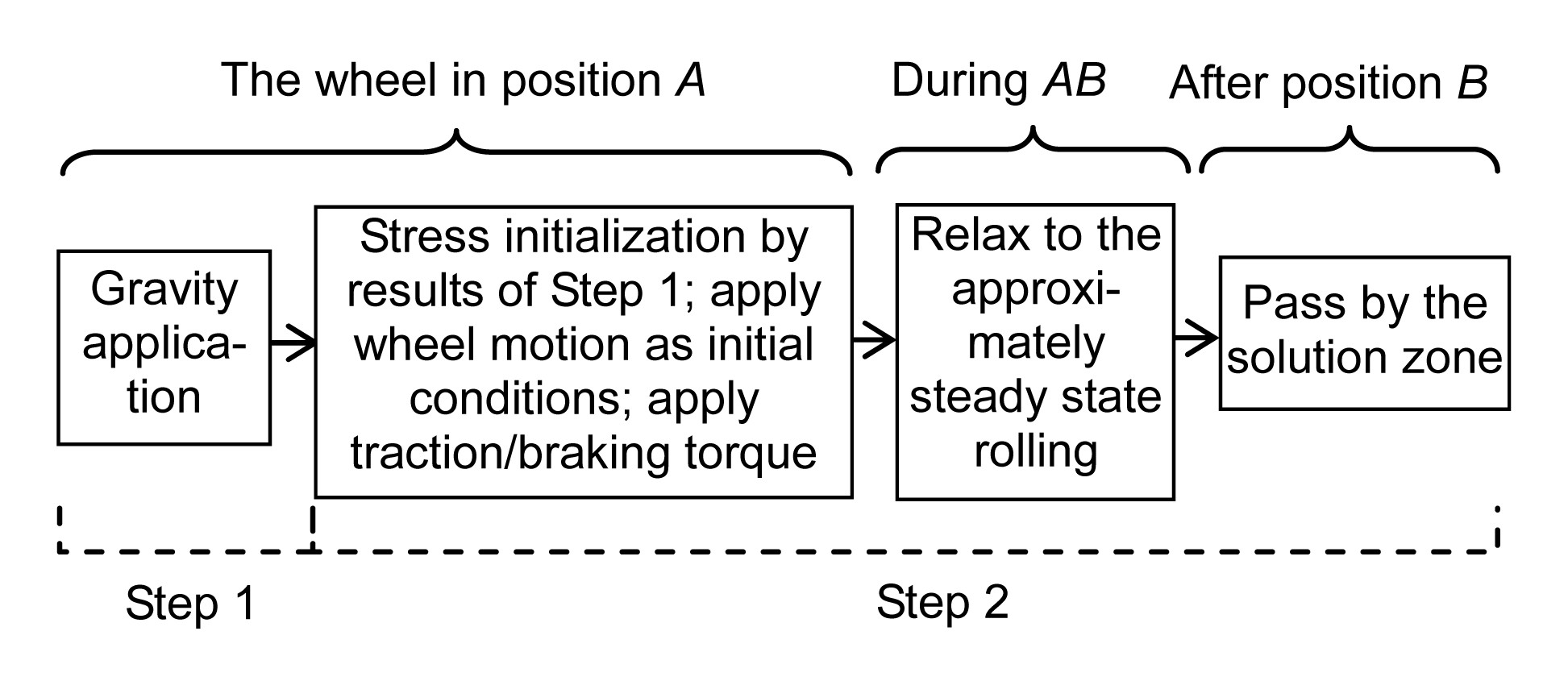
 The simulation is composed of two steps. Step 1: the static equilibrium state of the system under gravity is first solved by an implicit solver in the initial position of the wheel (position A in Fig. 2a). Step 2: an explicit solver is employed to simulate the transient rolling contact in the presence of friction, for which the displacement field obtained in Step 1 is used for stress initialization (at t=0), the predefined rotational and forward speeds of the wheelset are also applied at t=0 as initial conditions, and a specified acceleration or deceleration is further modeled by applying the time-dependent traction or braking torque to the wheel axle (M in Fig. 2b). The distance before the solution zone (i.e., AB in Fig. 2a) is designed to ensure that the wheelset achieves the steady state rolling approximately before entering the solution zone. When the wheelset passes by the solution zone, the transient results on forces, stresses, and strains are obtained. Such a process is sketched in Fig. 3. The determination of the distance AB is presented in Section 3.1. Note that the speed increase/decrease in the simulation caused by the torque M is negligible in comparison with the simulated speed because of the short time period simulated (typically 0.04 s) and, therefore, is ignored in later explanations.




 A central difference method based explicit scheme is employed to treat the time integration in Step 2. A very small time step (e.g., 8.9×10⁻⁸ s for the model in this study) is required to meet the Courant stability condition of the explicit solver or to ensure the convergence of the method. Because of such a tiny time step, the high-frequency dynamic behavior of the vehicle-track system and the transient rolling contact phenomenon can be captured effectively. Due to the high computational costs, only one wheel passage is simulated at present.

2.1.3.  Traction and creepage

 The coefficient of friction (COF, f), defined by Eq. (1), is reported to be typically 0.4–0.65 for dry-clean wheel-rail contact and less than 0.3 in the presence of a thin film of water or oil (Cann, 2006). In this study, the COF is taken as 0.5 (Table 1) to simulate the dry-clean condition. (1) , where F _T and F _N are the tangential and the normal (vertical) contact forces, respectively, transmitted through a full-sliding contact. Obviously, the maximum tangential load that can be transmitted through a wheel-rail contact is fF _N, i.e., in full-sliding contact, while a smaller load is transmitted in the case of rolling-sliding contact. 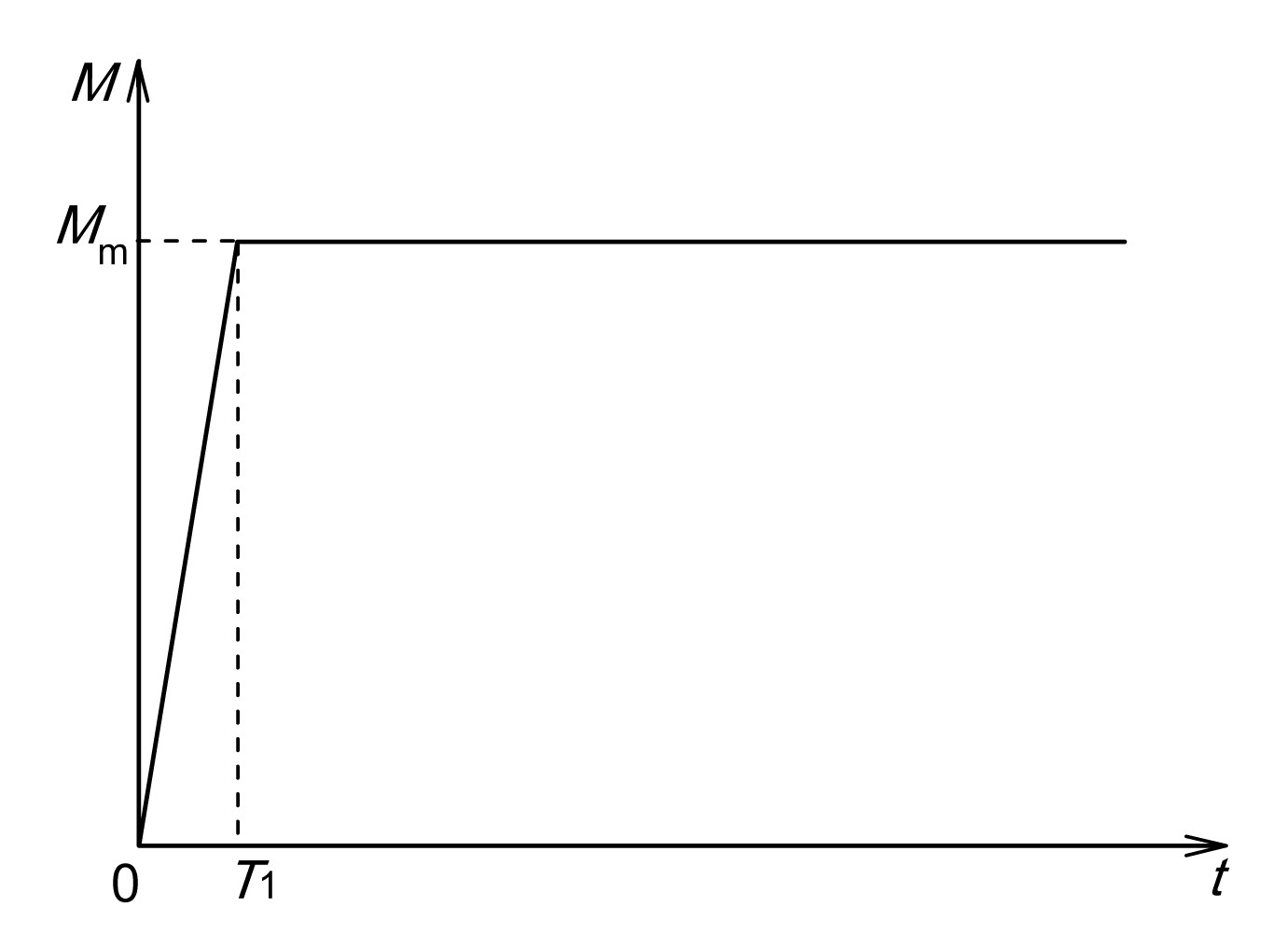Hereinafter, the tangential load actually transmitted is measured by a traction coefficient (μ) defined by (2) , where F _L is the longitudinal component of the tangential wheel-rail contact force, being the traction force for a driving wheelset in acceleration or the braking force for a wheelset in braking. Different traction/braking loads or different friction exploitation levels are simulated by specifying the corresponding driving torque M in the model. The torque M is assumed first to increase linearly from zero to its maximum and then remain constant (Fig. 4). Note that F _L is equivalent to F _T in this study because the tangential plane coincides approximately with the horizontal plane and no lateral friction force is considered.




 Referring to Fig. 5, the longitudinal creepage ξ corresponding to a specified traction load is calculated using (3) , where ω, R, and v are the angular speed around the axis, the radius of the wheel, and the translating speed, respectively, and ωR is the linear speed of a node in the wheel contact surface. Note that, traditionally, “creepage” is a concept defined by rigid motion, whereas elastic deformation is considered in this study. In Eq. (3) the linear speed of a node in the contact surface is taken as the linear speed of the wheel, through which the continuum vibrations excited by the contact load are considered in the calculated creepage.

2.1.4.  Material model

 A linear elastic material model is used for the wheel and the rail for the following reasons: (1) for steels, known as Hookean solids, the assumption of linear elastic behavior is valid in many cases (Meyers and Chawla, 1999); (2) shakedown is expected for most cases because of the generation of residual stresses and work hardening, which ensures the relatively long service lives of wheels and rails; (3) even at locations where plastic deformation occurs, its magnitude must be very small in each wheel passage, leading to a continuous increase of the rail surface hardness during the first two years after installation (Olofsson and Telliskivi, 2003). More accurate material models, once ready and if necessary, can easily be introduced. The slab and mortar materials are also assumed to be linear elastic.

 Material damping is considered by Rayleigh damping (C _m): (4) , where α and β are the mass (m) and stiffness (K) proportional damping constants, respectively. Trial simulations confirmed that the mass proportional damping is more effective for low frequency vibrations, and also damps out rigid body motions, as stated in the keyword user’s manual of LS-DYNA. Therefore, the mass proportional damping is not suitable for this work and only the stiffness proportional damping is employed. The value of β is chosen based on the estimate made by Kazymyrovych et al. (2010), in which β for an FE model was determined by matching the measured stress level during testing with the level calculated using the FE method.

2.2.  Frictional work and wear prediction

 The frictional work at a point of the rail contact surface (W _f) is calculated as (5) , where τ and s are the surface shear stress and micro-slip (i.e., the relative speed between contacting particles) at the point, respectively, being functions of time. τ_i and s_i correspond to the instant iΔt _W, the time step Δt _W is taken as 1×10⁻⁵ s (the wheel translates 0.83 mm within Δt _W at 300 km/h), and n _t is the number of calculated time steps. Material wear, if assumed to be proportional to the frictional work (Clark et al., 1988), can directly be scaled from the frictional work. More complicated/realistic wear behavior is beyond the scope of this work.

2.3.  Corrugation model

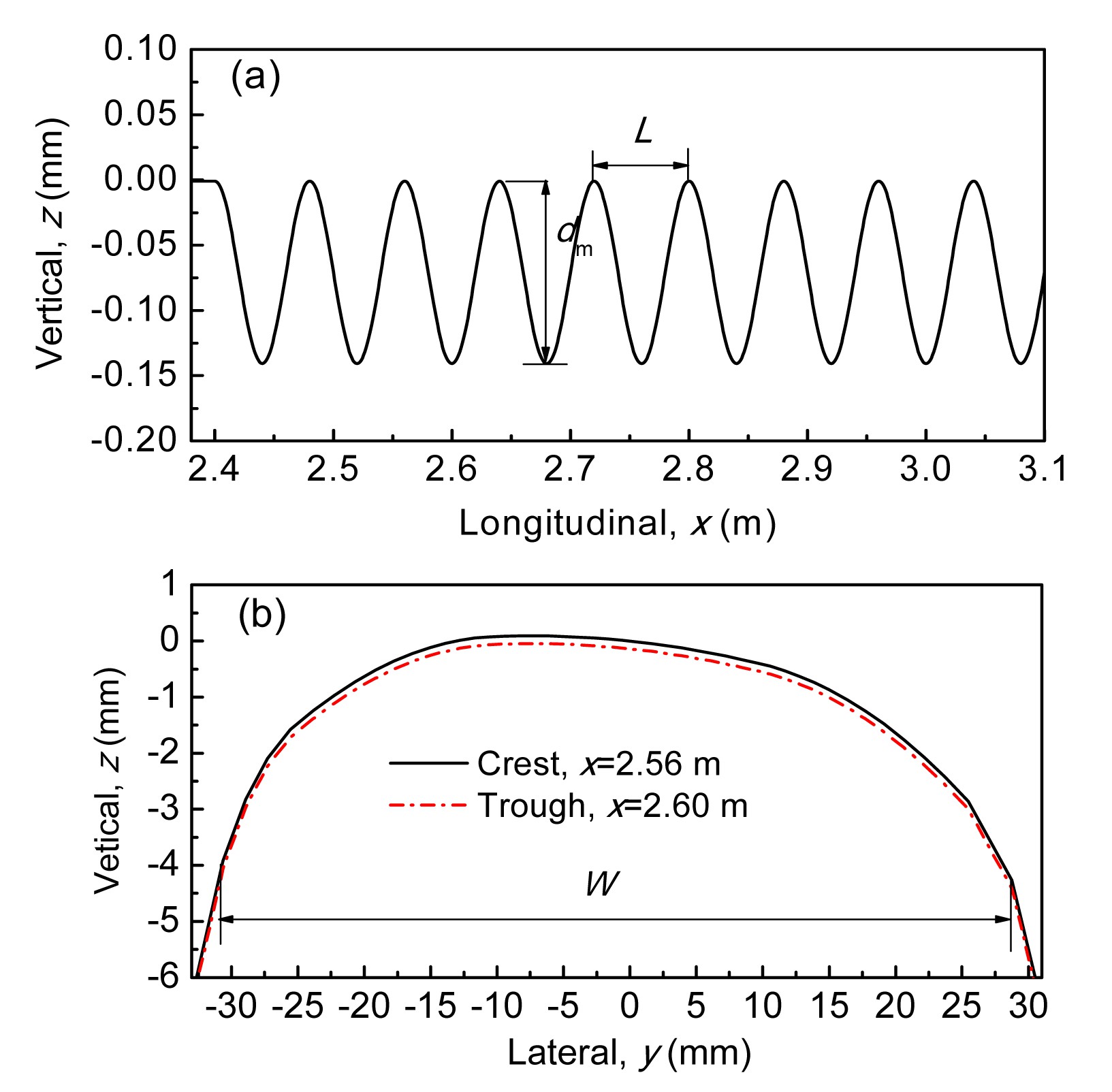
 Fig. 6 shows an example of the 3D corrugation models. The distribution of the corrugation depth (d) is assumed to be sinusoidal in the vertical-longitudinal section and parabolic along the lateral direction, as determined by (6) , (7) , where d _m, L, and W are the maximum depth, wavelength, and width of the corrugation, being 0.14 mm, 80 mm, and 30 mm for corrugation D (default), respectively; d _C is the maximum depth in the lateral direction and is located in the middle of the corrugation; x _s is the longitudinal coordinate at the starting point of the corrugation and is equal to 2.4 m. To maximize the influence of the corrugation for better analysis, d _C is applied to the position where the maximum contact pressure occurs in a case with smooth rail surfaces, i.e., in the vertical-longitudinal section of y=−2.8 mm (Fig. 17b). Note that the inclination of the rail is included in Fig. 6 and different scales are applied in Figs. 6a and 6b for clarity. The smooth case serves as a trial simulation for corrugation applications.

3.  Results of smooth contact surface

3.1.  Dynamic relaxation

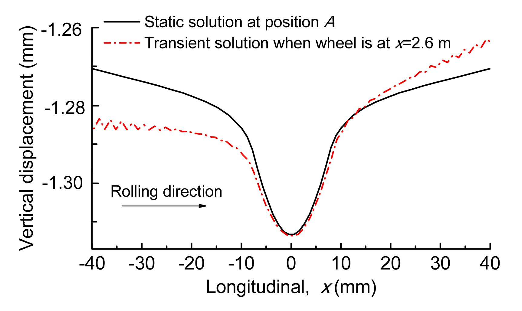
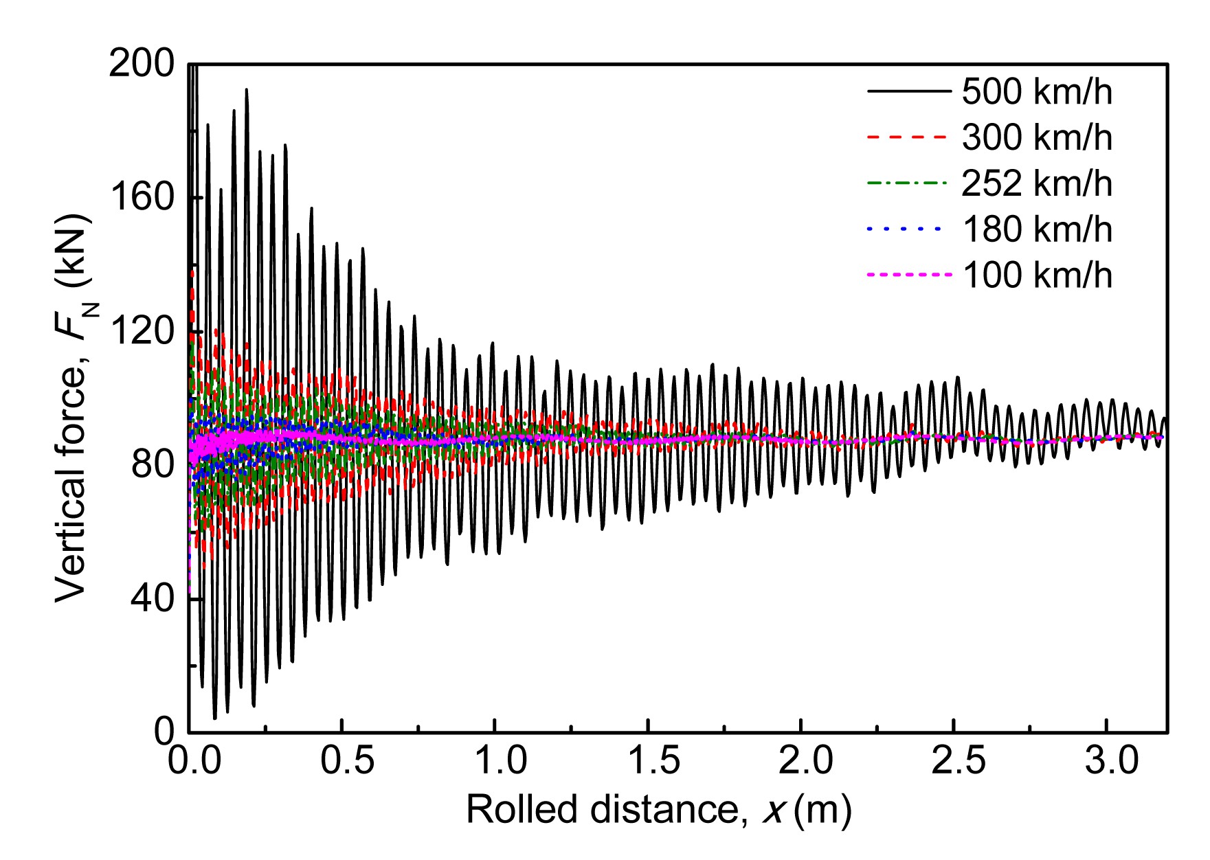
 It is mentioned above that the static solution obtained by the implicit solver is employed to initialize the transient simulation. Fig. 7 shows that the vertical displacement field of the rail surface is symmetric in the vicinity of the contact patch in the static case, while it becomes asymmetric in the transient analysis due to the moving load. Hence, when the wheel rolls forward in a transient analysis, the displacement field gradually changes from the static to the transient case. Such a process inevitably introduces an oscillation (referred to later as the initial oscillation), as observed from the vertical (contact) forces plotted in Fig. 8. Note that Fig. 7 shows the results only along a longitudinal line where the maximum pressure is, i.e., the longitudinal axis of the contact patch when the contact patch is an ellipse. More studies have shown that the influence of the rolling speed on the pressure distribution is negligible in the case with a smooth rail contact surface. This is because the resultant speed at the contact point (assuming a rigid contact, the contact patch reduces to a point) is zero, being independent of the rolling speed, i.e., the instantaneous center of the wheel. Hereinafter, the longitudinal line is referred to as the longitudinal axis, although the contact patch is not necessarily an ellipse, e.g., on corrugated rails. Results shown later are all taken from the rail side.







 From Fig. 8 it is seen that AB (Fig. 2a), designed for a dynamic relaxation, should be at least 2.4 m long for the system to relax to an acceptable oscillation level (10% of static load) in position B at 500 km/h. This is how AB was determined. For a speed under 300 km/h, the vertical force becomes very stable after a rolled distance of 2.4 m. Note that the abscissa of Fig. 8 is set to be the rolled distance for comparison.

 Note that the displacement difference in Fig. 7 may not be the only reason behind the initial oscillation. Other factors, probably related to the initial conditions, may also play certain roles. Nevertheless, this is not discussed further because this study focuses on the contact solution after achieving an approximate rolling state.

3.2.  Longitudinal and vertical forces

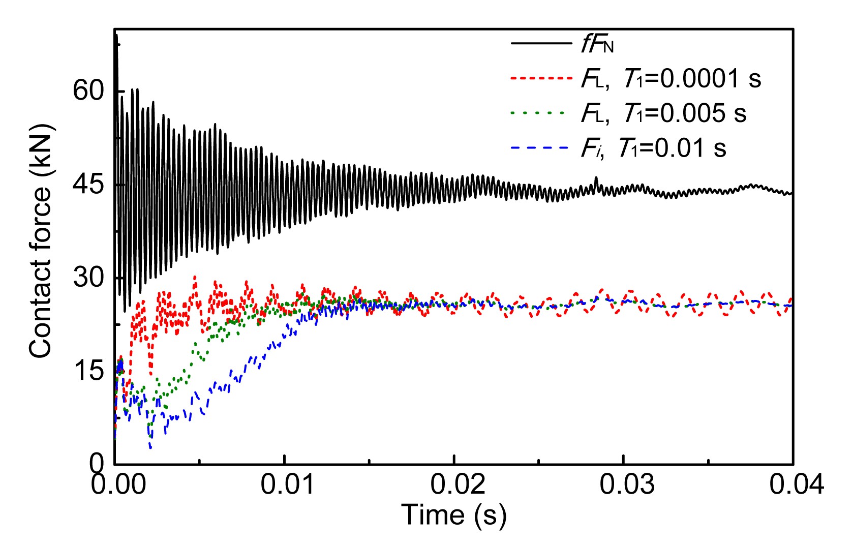
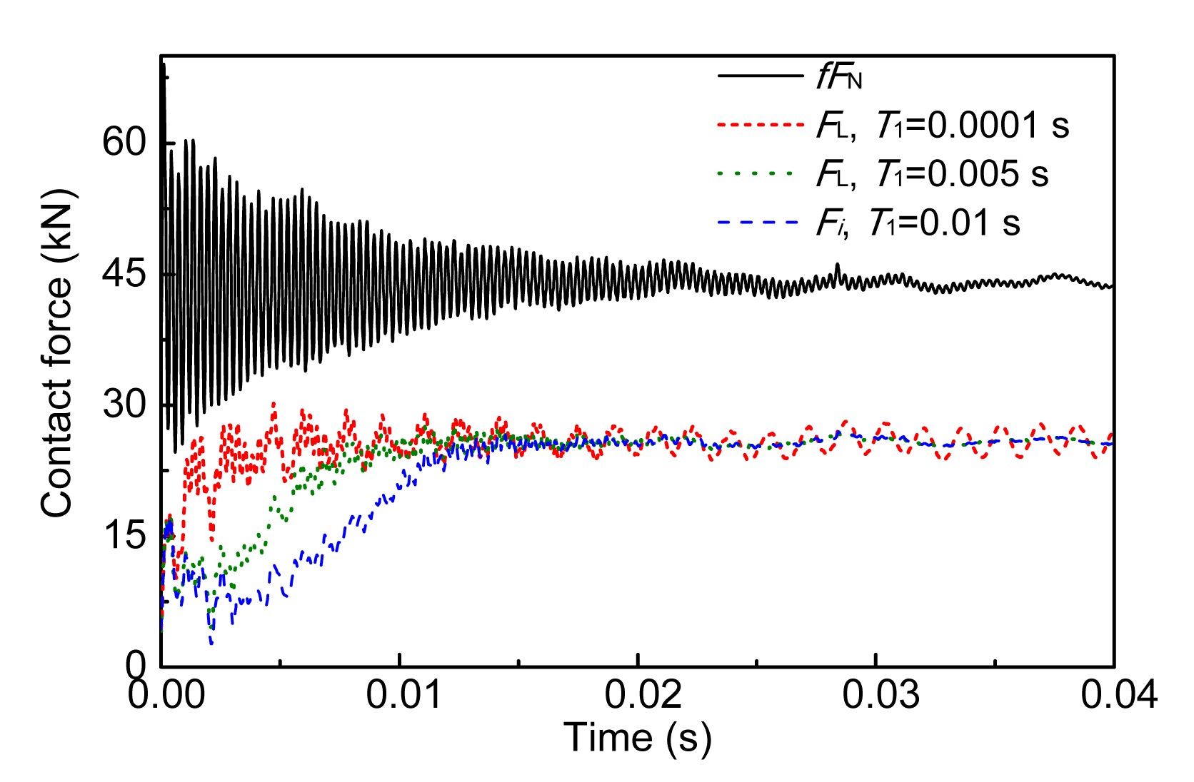
 The initial increase rate of the driving torque is varied by setting T ₁ (Fig. 4) at different values, from zero to sufficiently large. Fig. 9 shows the contact force results of a smooth case when T ₁ is varied, for which a rolling speed of 300 km/h and a traction coefficient of 0.3 are assumed. For clarity, only representative results corresponding to three values of T ₁, namely 0.0001, 0.005, and 0.01 s, are plotted. As expected, the vertical force does not change considerably with T ₁ (a difference of much less than 1%). Hence, only one vertical force result scaled by the COF (i.e., fF _N) is plotted in the figures to illustrate the limit of the longitudinal force.




 The initial oscillation also influences the longitudinal (contact) forces considerably (Fig. 9). After the dynamic relaxation (t>0.028 s), the longitudinal force becomes very stable, like the vertical force, when T ₁ is 0.005 or 0.01 s, but not in the case when T ₁=0.0001 s. Moreover, the longitudinal force does not reach the specified value at T ₁ but has a delay of about 0.005 s. This delay is the response time of the material in contact to the torque applied to the axle. Hereinafter, cases with T ₁=0.005 s are used for analyses. Variations of the longitudinal force in the case with T ₁=0.0001 s are not further studied here.

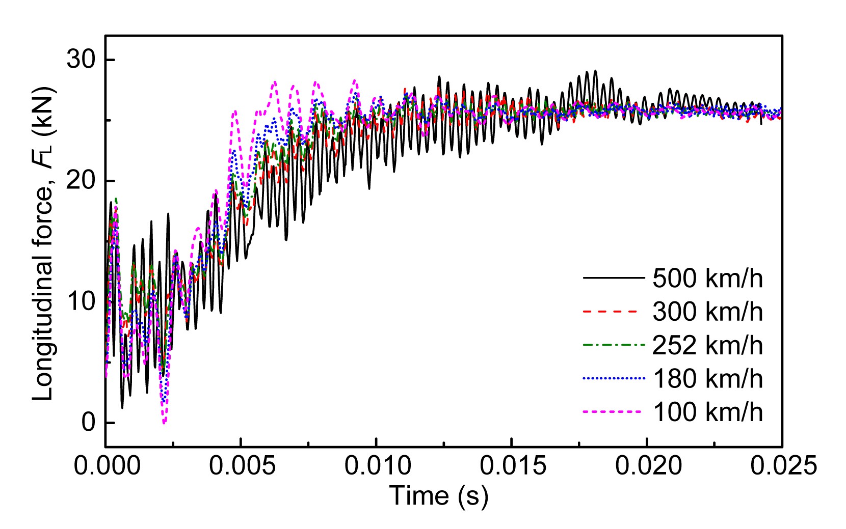
 Contact force results at different rolling speeds and with different traction coefficients are shown in Figs. 10 and 11, respectively. A stable rolling contact is achieved after the dynamic relaxation in all cases.

3.3.  Contact stresses and frictional work

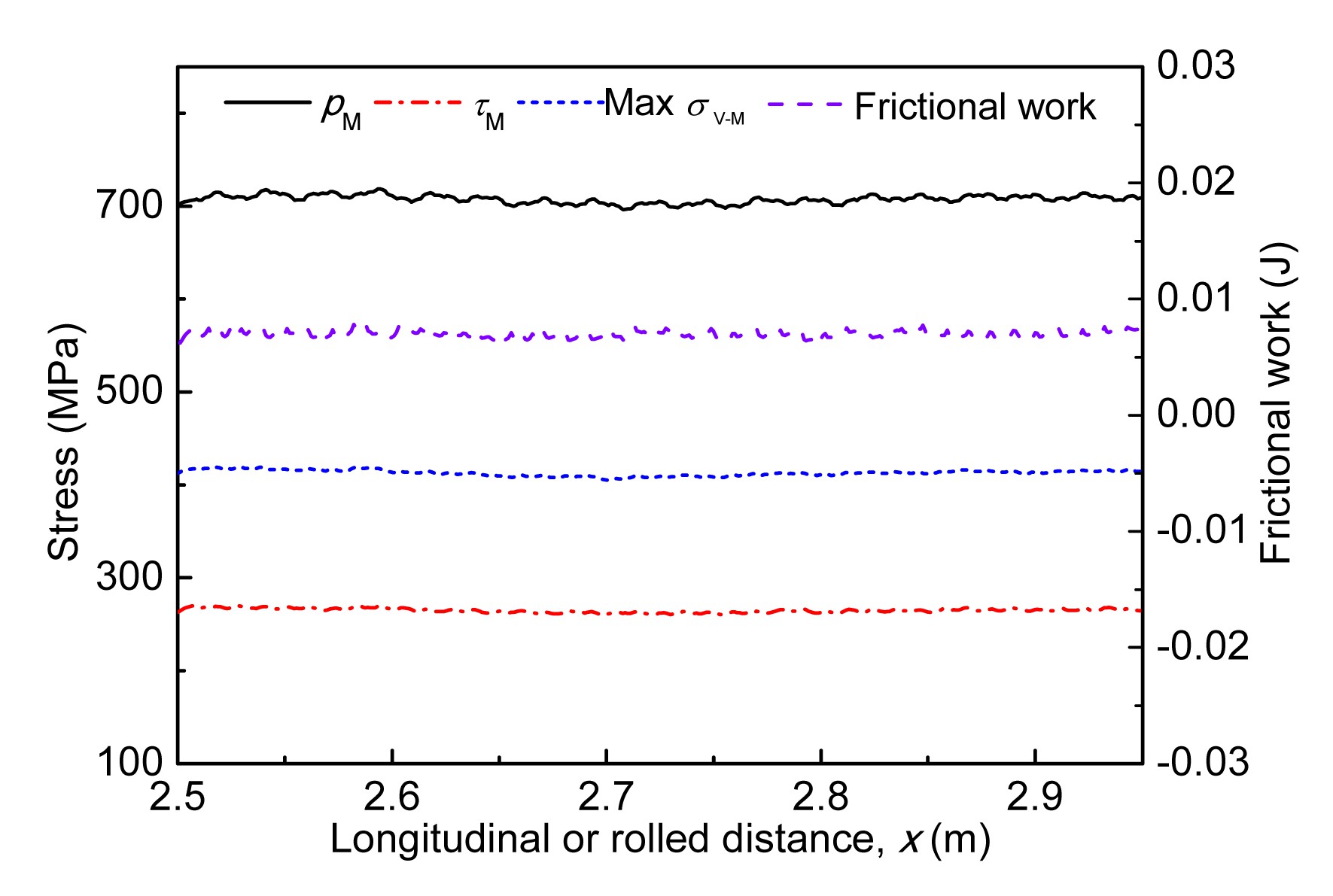
 For the case of v=300 km/h and μ=0.3, distributions of the maximum contact stresses along the longitudinal axis are shown in Fig. 12 together with the corresponding frictional work. A maximum stress at a location means the maximum value reached at that location during the simulated wheel passage. The frictional work given in the figure indicates the calculated result in a longitudinal strip with a width of 1.1 mm (the width of the elements there). These results confirm that approximately steady rolling is achieved in the simulation.




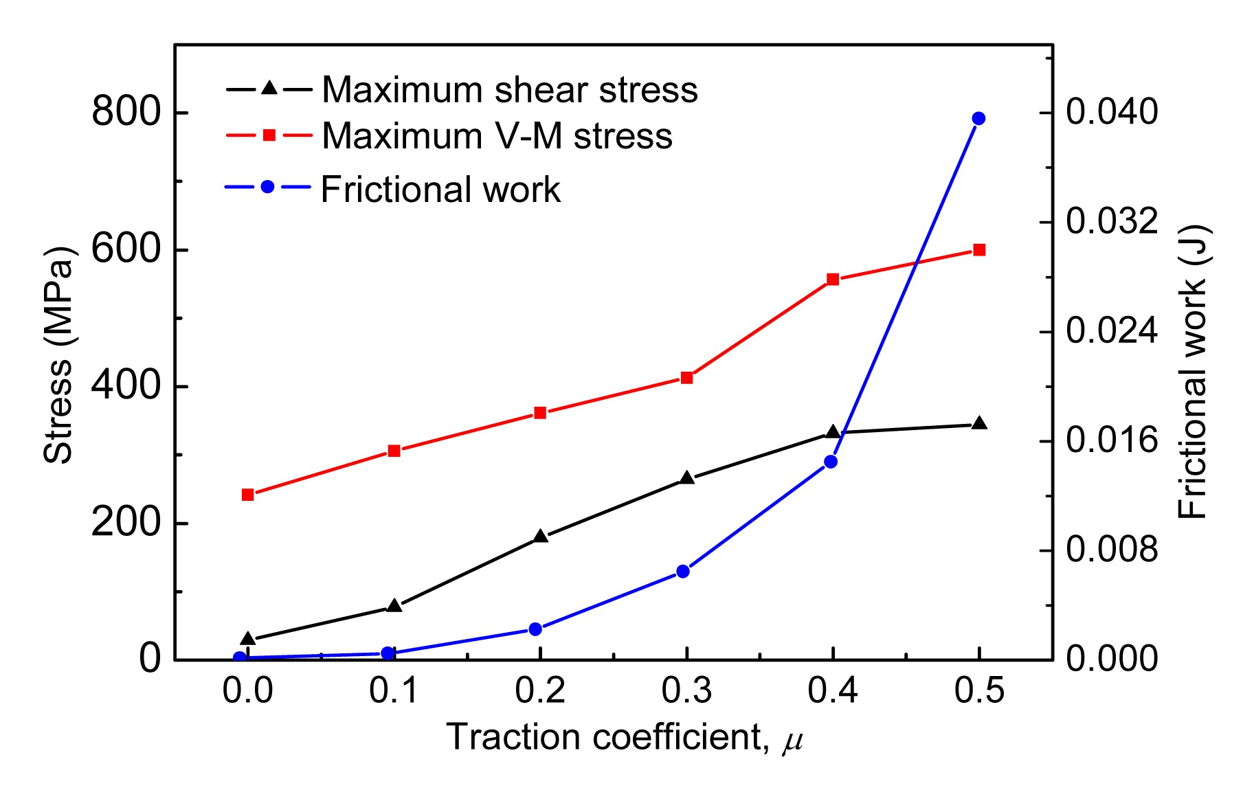
 As the traction coefficient becomes larger, the magnitudes of the stresses and frictional work shown in Fig. 13 all increase, as expected. Note that the Von Mises (V-M) stresses presented in this study are of the surface layer of elements (at their centers) because constant stress elements are employed. Pressure is not plotted in Fig. 13 because it is independent of the traction level.

4.  Corrugation

4.1.  Measurements on a high-speed line

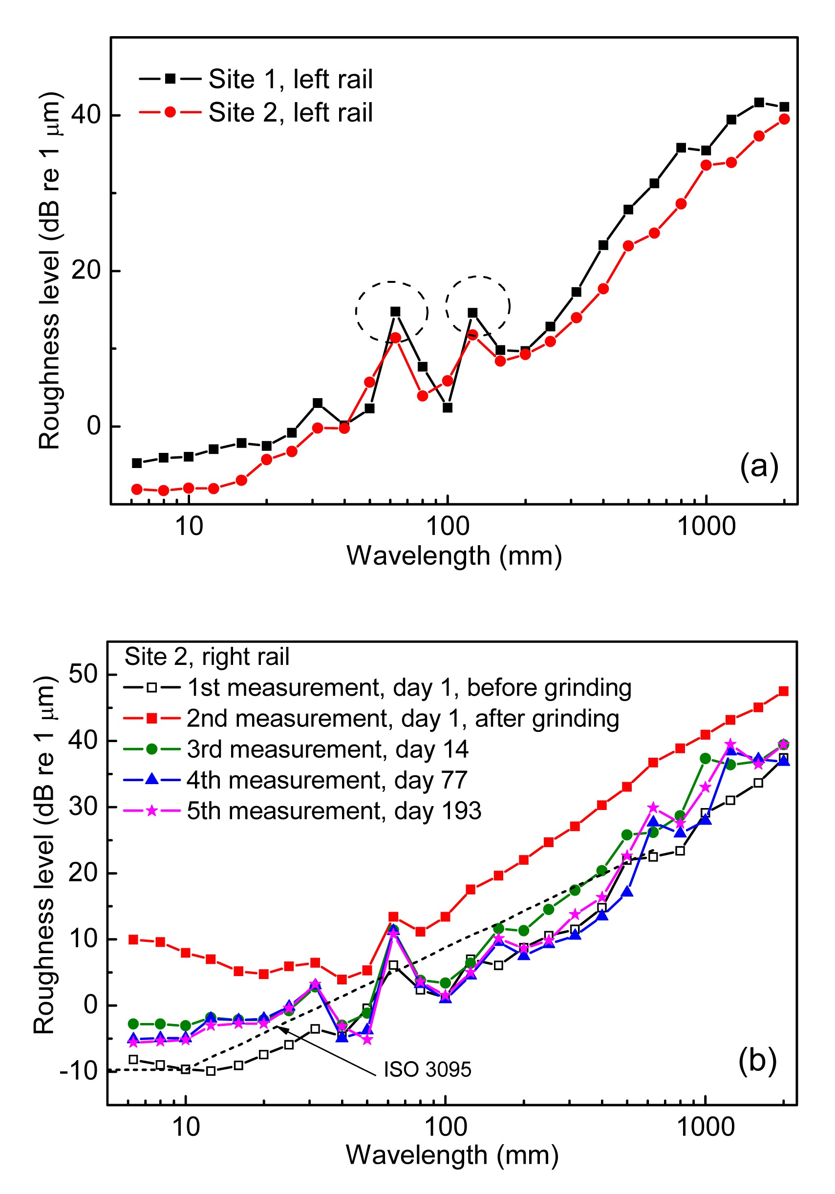
 Corrugation occurred on a Chinese high-speed line was measured using a corrugation analysis trolley (CAT). Fig. 14a shows roughness level spectra in 1/3 octave bands measured at two sites where the running speeds were about 300 km/h. Two typical wavelengths, namely around 65 and 125 mm, are observed and the first one dominates. Note that the wavelength of 80 mm shown in Fig. 1 (a picture taken on site 2 illustrated in Fig. 14) is not obvious in the roughness level spectra. This may be because those spectra were obtained from measurements of rails of several hundred meters (about 300 and 1000 m at sites 1 and 2, respectively), in which the wavelength of the corrugation varied around 65 mm and the wavelength of 80 mm existed at only some locations. The physical essence behind such a wavelength variation is likely to be the inevitable variations of the vehicle-track parameters along the measured site. In addition, the discrete frequencies taken in the 1/3 octave bands may also cause some errors in the wavelength estimation. Fig. 14b shows five CAT measurements at site 2 conducted during a grinding cycle. It is seen that the corrugation re-occurred after grinding and gradually became stabilized in a short period.




 In this study, corrugation with a wavelength range of 65–95 mm is modeled to study its influence on transient wheel-rail interaction at high-speeds. All corrugation models are applied in the same way as corrugation D (with the default wavelength of 80 mm, Fig. 6), i.e., with the same location and phase in the longitudinal direction, and the same depth distribution in the lateral direction. Other corrugation models are later referred to by their wavelengths and maximum depths, without presenting their geometry in figures.

4.2.  Transient wheel-rail interaction

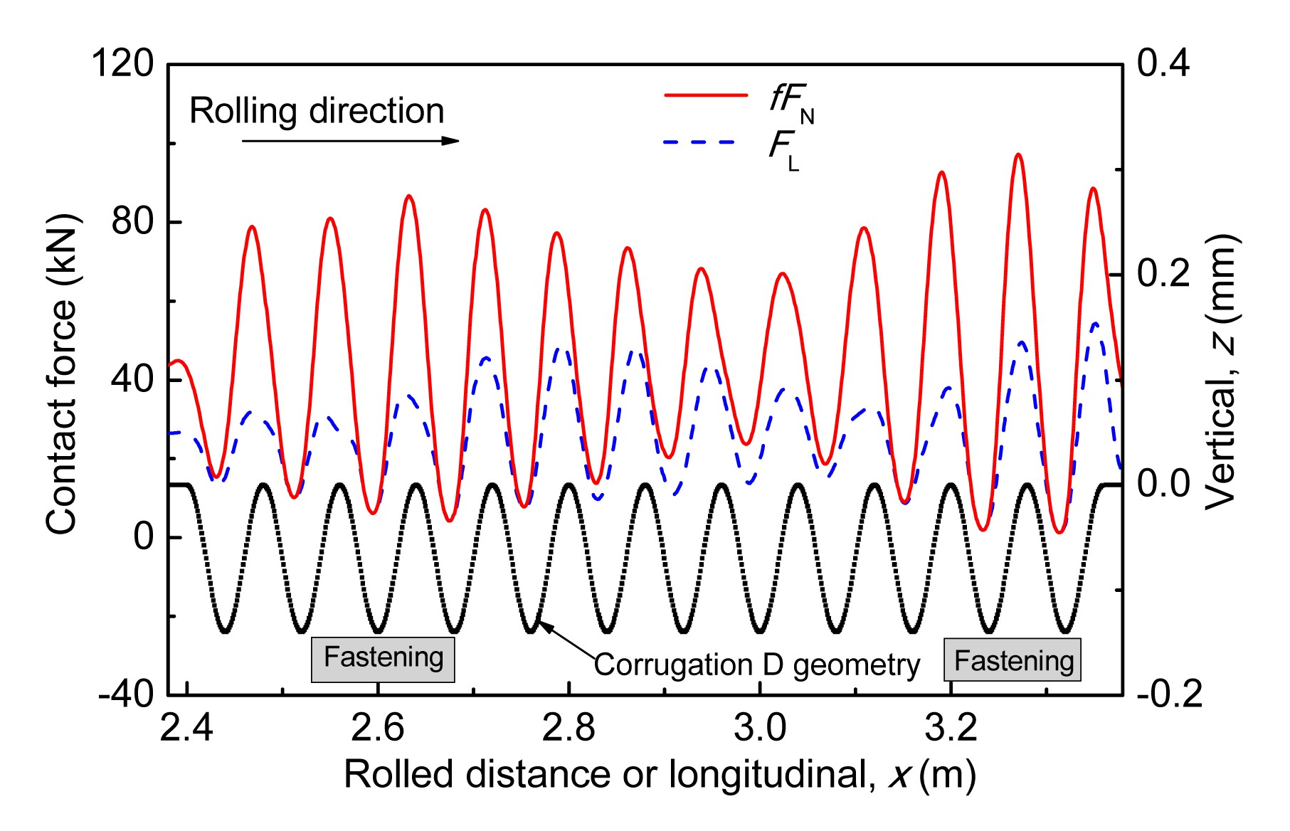
 The transient wheel-rail interaction on a corrugated rail is analyzed in this section, for which corrugation D is considered with v=300 km/h and μ=0.3. Fig. 15 shows variations of the contact forces together with the geometry of corrugation D, in which the vertical force is scaled by the COF (f) for comparison. As expected, both the vertical and longitudinal forces significantly fluctuate at the corrugated site. The maximum vertical force (F _N) is 193.19 kN and the minimum is as low as 3.02 kN, i.e., the wheel and rail almost separate from each other. At several corrugation troughs fF _N coincides with F _L, i.e., full sliding occurs. The phenomenon that the force peaks do not occur exactly at the corresponding corrugation crests (referred to as the longitudinal shift hereinafter) will be discussed later.




 Furthermore, the vertical force is larger when the wheel is above the fastenings than in between, demonstrating the considerable influence of the discrete supports of the rail. Such a result is in line with authors’ observations that some corrugations are deeper in positions above fastenings than in between, which has also been reported in (Clayton and Allery, 1982; Jin et al., 2008). Note that the influence of the discrete supports on the longitudinal force is different from that on the vertical one. The relationships between the normal and the tangential wheel-rail interactions will be discussed later.

 Pressure and surface shear stress distributions at 10 typical instants (i.e., t1–t10) are plotted in Fig. 16 to show the transient effects. As expected, the contact stresses vary greatly on the corrugated rail. Within the selected instants, the rolling contact changes from the rolling-sliding state to full sliding (at t4), and then back to rolling-sliding. It should be specified that the pressure reaches local maximums (within a wavelength) at t1 and t7, and local minimums at t4 and t10. At t1, t7, and t4 the surface shear stress also reach local maximums or minimums, but another local minimum occurs at t10′, being slightly different from t10. In a word, the typical instants are not completely the same in Figs. 16a and 16b for better illustration.




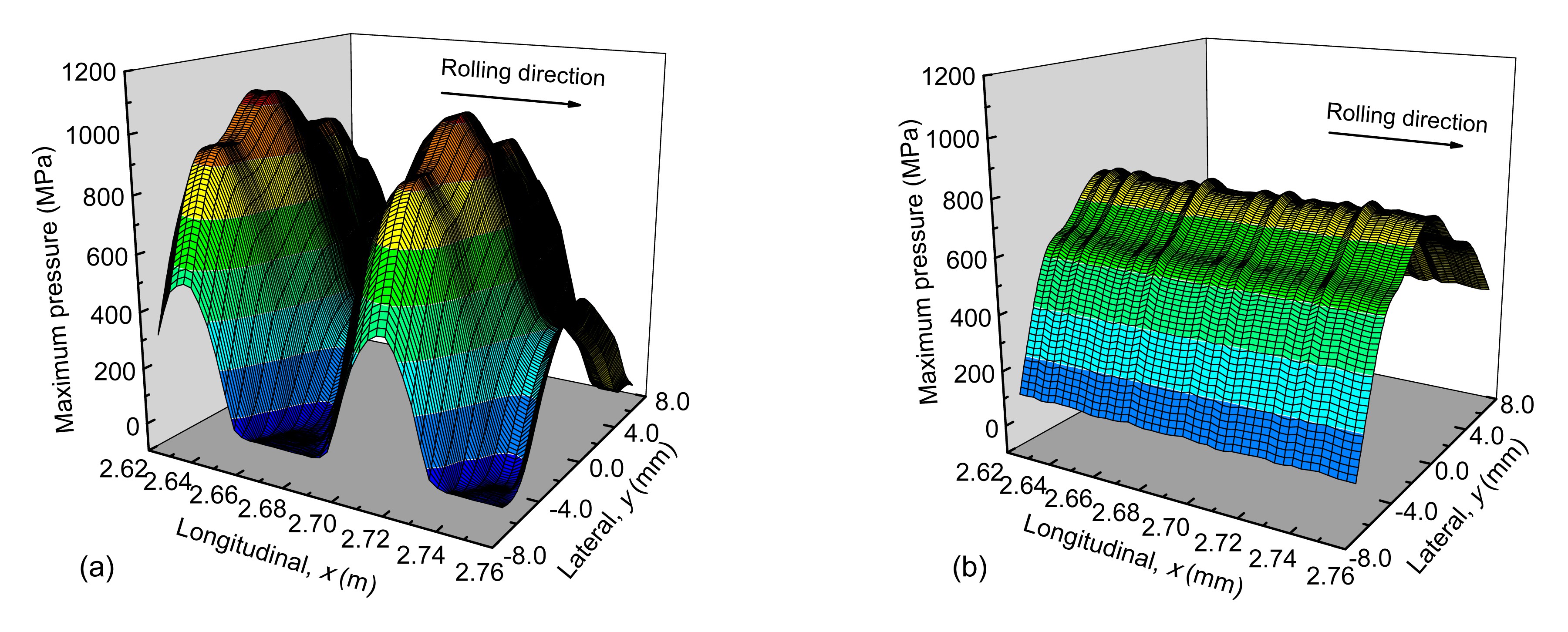
 It is further seen from Fig 16a that local maximums of pressure occur before the contact patch center reaches a corrugation crest. This is because the pressure is determined by both the contact geometry and the dynamic vertical force (as mentioned above, a longitudinal shift exists). Fig. 17a shows the 3D distribution of the maximum pressure in the same section as in Fig. 16. Comparing Fig. 17a with the corresponding results on the smooth rail shown in Fig. 17b, great influences of corrugation can be observed clearly.




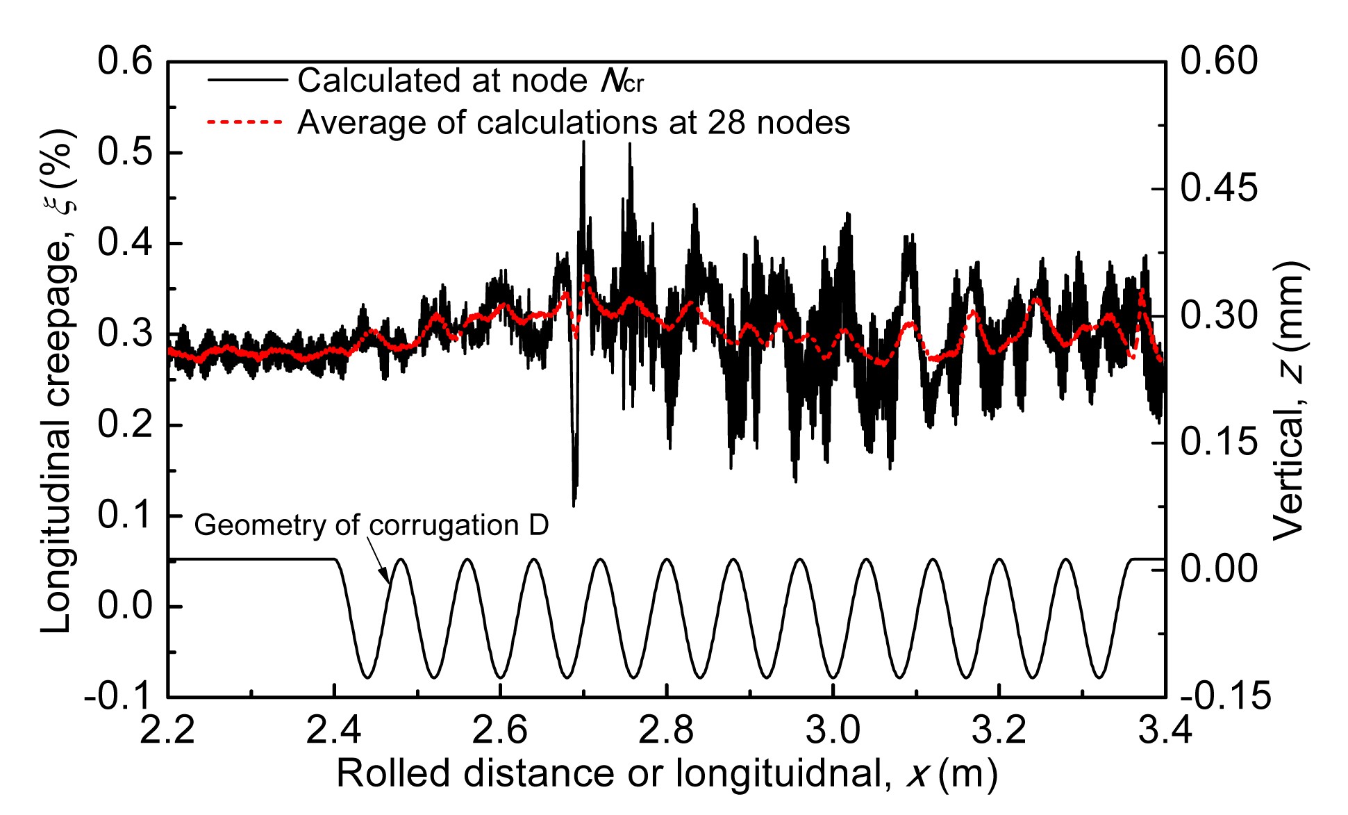
 Fig. 18 presents the creepage variation caused by corrugation D. From the creepage results calculated at node N _cr (located in the contact patch at t=0, Fig. 5) it is seen that the maximum creepage reached on the corrugated rail is close to double the stabilized value on the smooth contact surface (before the wheel enters the corrugation, about 0.276%). Fluctuation of the creepage becomes obviously fiercer at x=2.69 m because the node N _cr comes into contact again after a rolled distance of 2.69 m (a cycle), i.e., continuum (local) vibrations are excited by the contact load. To filter out the influence of the local vibrations, the calculated creepages at 28 selected nodes (distributed over the whole circumference of the wheel) are averaged and also plotted in Fig. 18. Little further explanation of the creepage results is given hereinafter because: (1) the transient contact stresses and the resulting irregular frictional work and/or irregular V-M stress, not the irregular creepage, are the immediate causes of corrugation development; (2) according to rolling contact theories, higher creepage usually means larger tangential contact force, higher frictional work, and larger V-M stress, which is valid for cases simulated in this study.




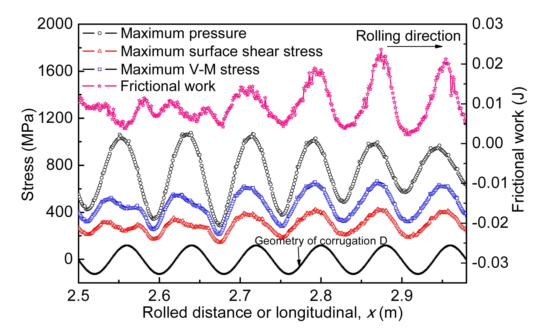
 Fig. 19 shows distributions of the maximum pressure, maximum surface shear stress, maximum V-M stress, and frictional work along the longitudinal axis in the corrugated section. It is observed that the stresses all vary following the pattern of corrugation, but with slightly different longitudinal phases, and the relative positions of the stress peaks with respect to the corresponding crests change slightly at different waves of corrugation. Moreover, the patterns of the maximum V-M stress and the frictional work are closer to that of the maximum surface shear stress than to that of the maximum pressure, as expected.

4.3.  Different wavelengths and depths

 Keeping v=300 km/h and μ=0.3, the wavelength (L) and depth (d _m) of corrugation are varied separately to study their influences. Considering the wavelength range reported in Section 4.1, three wavelengths, namely 65, 80, and 95 mm, are considered. Fig. 20 shows that among the simulated cases, the maximum vertical and longitudinal forces both occur in the case of L=80 mm. For L=65 mm, the longitudinal force does not follow the pattern of the simulated corrugation any more, but shows a shorter characteristic wavelength (Fig. 20b), and its magnitude is much smaller than in the other two cases. This may be explained as follows: the excitation frequency of corrugation (f _ex=v/L, i.e., the passing frequency) monotonically decreases with the corrugation wavelength; for a wavelength of 80 mm, f _ex is closest (among the three cases) to an eigen-frequency of the system related to corrugations, leading to the strongest response.




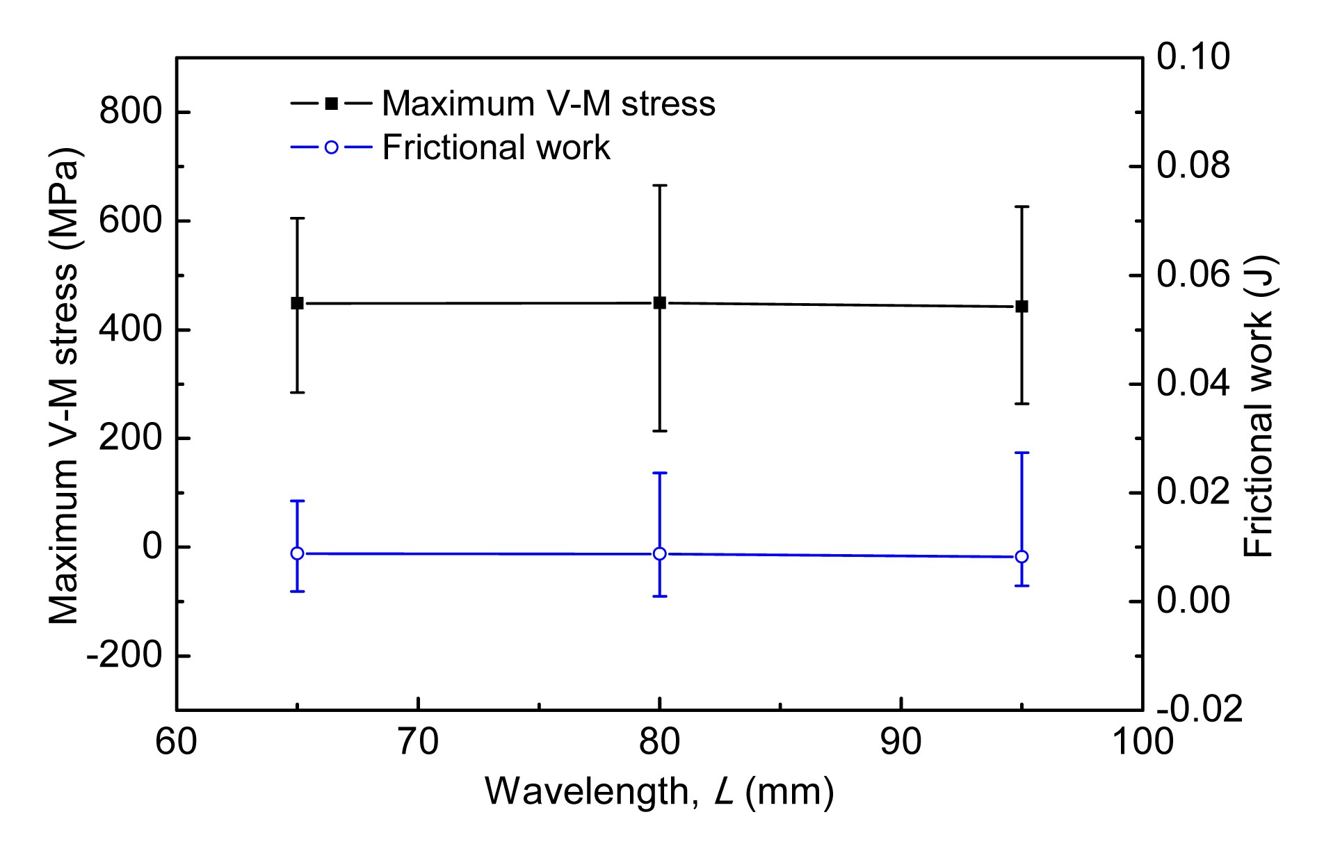
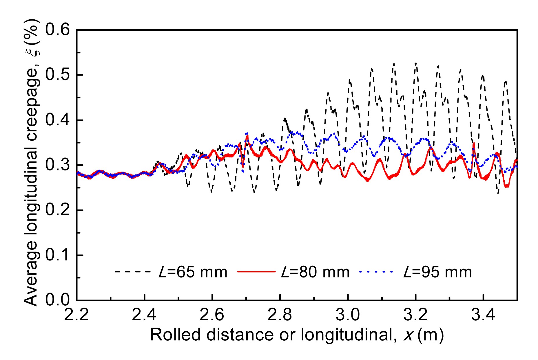
 The mean value of the maximum V-M stress in the corrugated section is approximately constant for different wavelengths, while its fluctuation range is the largest at L=80 mm (Fig. 21). This is in line with the longitudinal force results in Fig. 20b. In contrast, the largest fluctuation of the frictional work occurs at L=95 mm (being 0.016, 0.023, and 0.024 J at L=65, 80, and 95 mm, respectively), because the frictional work is determined not only by the contact stresses (or the contact forces) but also by the micro-slip. Significant influences of the wavelength on the micro-slip in the corrugated section can be seen from the creepage (integration of the micro-slip over the contact patch) variations given in Fig. 22. No more detailed distributions of the maximum V-M stress and the frictional work in corrugated sections are given hereinafter, considering that their patterns are similar to that of the longitudinal force, as mentioned above.







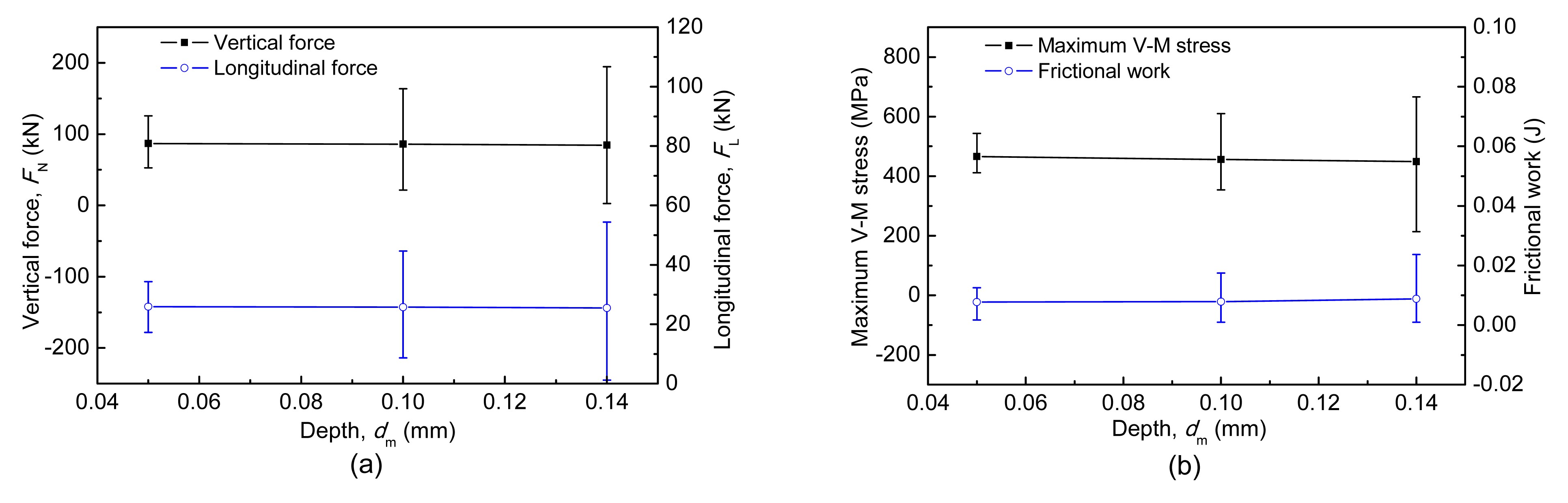
 When the corrugation depth increases, fluctuation ranges of the dynamic forces, the maximum V-M stress, and the frictional work all increase as expected (Fig. 23). Detailed variations of the dynamic forces are not illustrated here because their patterns remain constant for different depths.

4.4.  Different traction coefficients

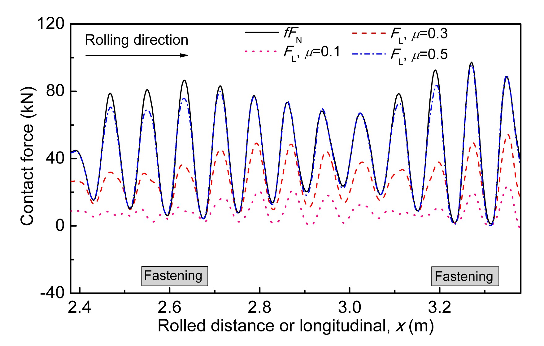
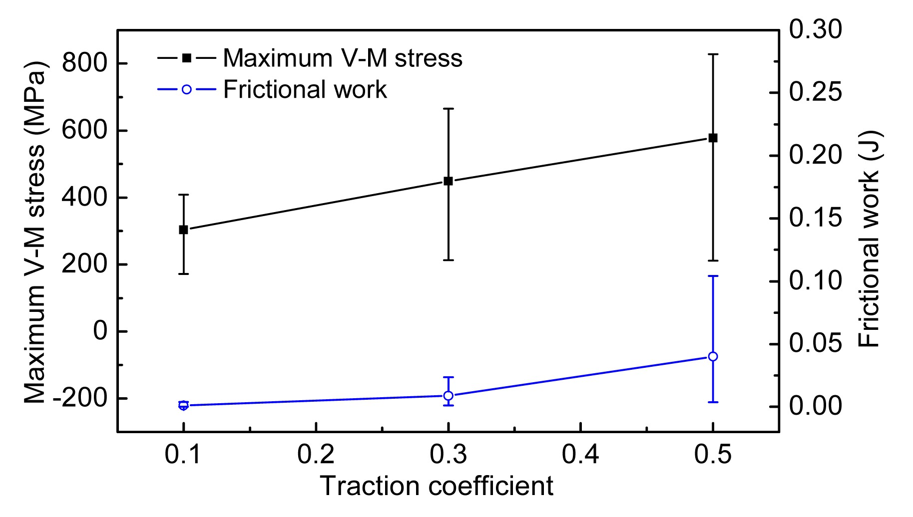
 The traction coefficient is varied from 0.0 to 0.5 to examine its influence on the tangential wheel-rail interaction, for which corrugation D is considered and the rolling speed is kept at 300 km/h. From the dynamic forces shown in Fig. 24 it is found that the longitudinal force gradually becomes in phase with the vertical force scaled by the COF as the traction coefficient increases. This is determined by Coulomb’s law of friction employed in the model, i.e., the surface shear stress distribution approaches the scaled pressure distribution with the increase of traction coefficient. When the traction coefficient is very low, variation of the pressure distribution (i.e., variation of the upper limit of the surface shear stress distribution) has little influence on the surface shear stress distribution since the slip area in the contact patch (where the upper limit is reached) is very small. Obviously, such an influence becomes more significant as the slip area enlarges, i.e., as the traction coefficient increases. This is why the fluctuation range of the longitudinal force increases with the traction coefficient (Fig. 24). Fig. 25 presents the mean values and fluctuation ranges of the maximum V-M stress and the frictional work over the section in Fig. 19. It is seen that the mean values and the fluctuation ranges all increase with the traction coefficient, showing the same trend as the longitudinal force.

4.5.  Different rolling speeds

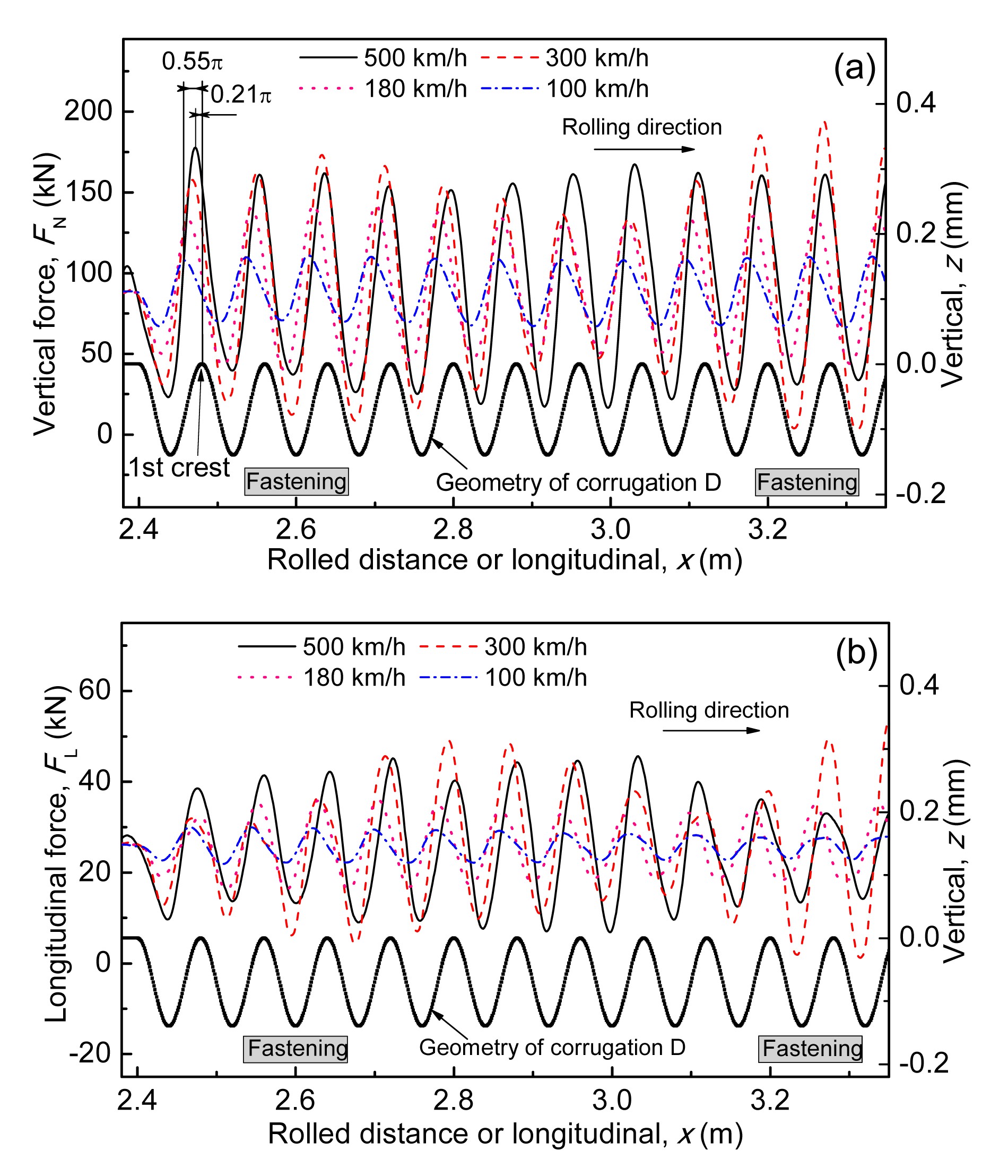
 The dynamic forces caused by corrugation D at different rolling speeds are illustrated in Fig. 26, in which the traction coefficient remains 0.3. The maximum vertical and longitudinal forces first increase with the rolling speed when the speed is less than 300 km/h, and then decrease (i.e., the maximums at 500 km/h are lower than those at 300 km/h). This is a consequence of the following phenomena: (1) the excitation frequency of the corrugation changes with the rolling speed, leading to the strongest response at a certain speed (the same reason as that mentioned in Section 4.3); (2) among the simulated speeds, the influence of the discrete supports of the rail is the greatest at 300 km/h (Fig. 26).




 Furthermore, the longitudinal shift of the vertical force decreases with the rolling speed. For example, as indicated in Fig. 26a, it varies from 0.55π at 100 km/h to 0.21π at 500 km/h at the first corrugation crest (a shift of 2π corresponds to a corrugation wavelength). Note that the relative positions of the force peaks with respect to the corresponding crests are not constant at different waves due to the transient effects.

 Influences of the speed on the longitudinal shift of the longitudinal force are more complicated than those of the vertical force (comparing Figs. 26a and 26b). This is because the tangential interaction has its own eigen-modes, and in the meantime is limited by the normal one. As mentioned in Section 4.4, the tangential force will follow exactly the vertical force scaled by the COF in a full sliding case due to the application of Coulomb’s law of friction.

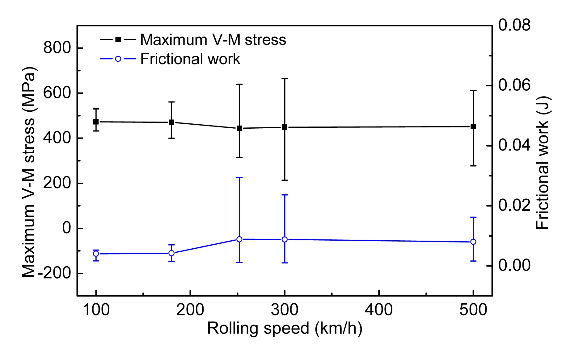
 From Fig. 27 it is further seen that the fluctuation range of the maximum V-M stress caused by corrugation D is the largest at 300 km/h, while at 250 km/h the fluctuation range of the frictional work reaches its maximum. From the results in Figs. 26 and 27 it could be concluded that, for the simulated speed range, the responses of the system to corrugation D reach the maximum at a speed between 250 and 300 km/h. Moreover, Fig. 27 shows that the mean values vary considerably when the rolling speed changes from 180 to 250 km/h.

4.6.  Comparison with the multi-body approach

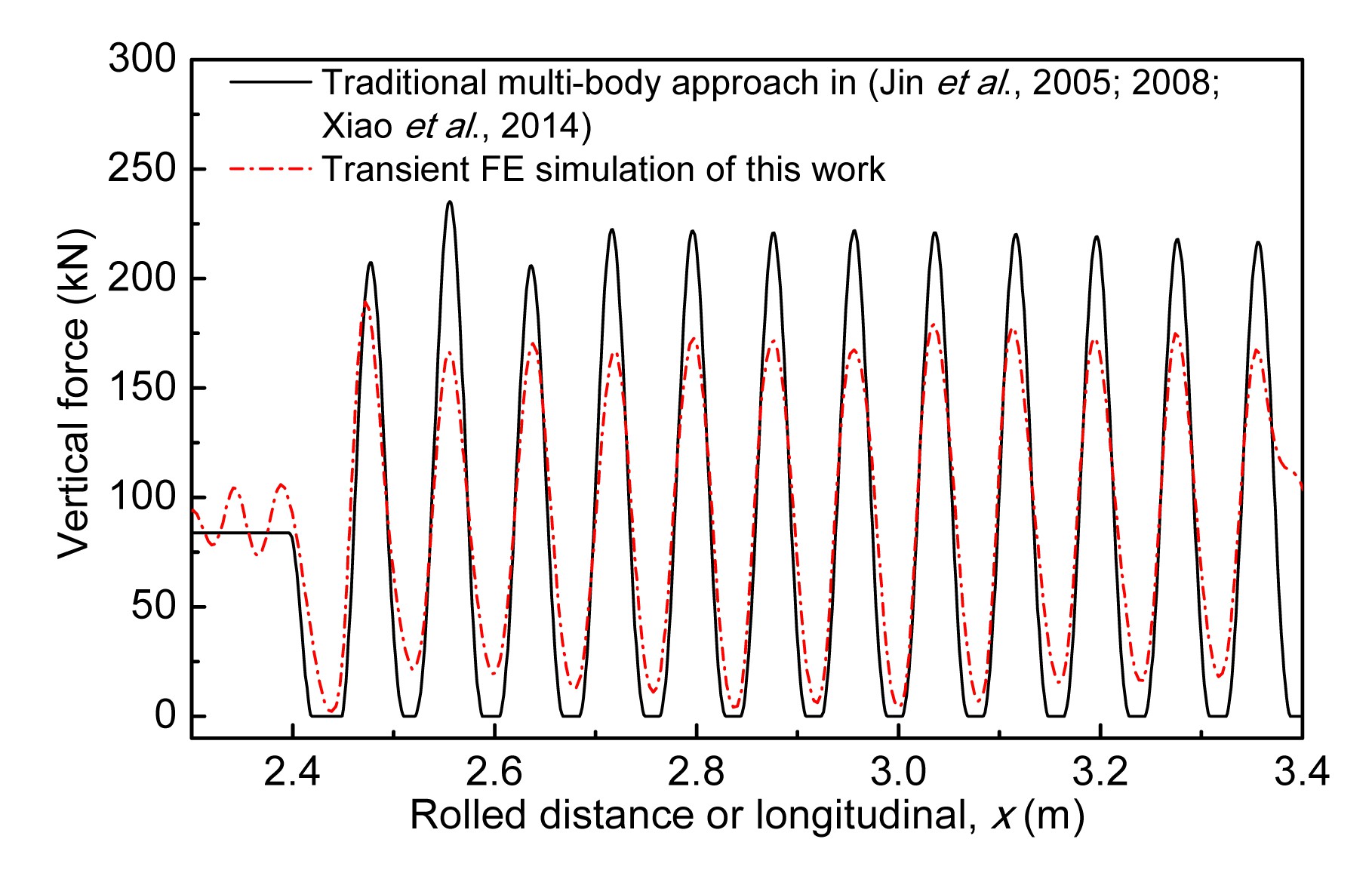
 The vertical force obtained from the transient FE simulation is compared to that of the traditional multi-body approach (Jin et al., 2005; 2008; Xiao et al., 2014) in Fig. 28, for which a corrugation with a wavelength of 80 mm and a depth of d _m=0.18 mm is considered at 500 km/h. It is seen that the transient FE result is significantly lower. Contact loss corresponding to the vertical force of zero is predicted by the multiple-body approach, but not by the transient FE simulation. Such a difference can be explained as follows: in the multi-body approach, the whole wheel is lumped into one mass particle, the rail is represented by Euler beams and a Hertz spring is used to model the wheel-rail contact, which significantly exaggerates the contact stiffness and assumes the contact patch is infinitesimal. In other words, the results from the transient FE model should be more reasonable and the multi-body approach overestimates the dynamic wheel-rail interaction under the excitation of corrugations. Note that the longitudinal force is not compared here because it cannot be obtained by the traditional multi-body approach.




 It should be specified that with a modified Hertz spring the traditional multi-body approach may still provide accurate predictions of the contact forces caused by corrugations. Such an approach is appealing due to the low computational costs of multi-body simulations. To this end, the transient FE model developed in this study provides a potential calibration and validation tool for the suitable contact stiffness. Once calibrated and validated, more accurate contact force predictions may be realized without increasing the computational costs.

5.  Discussion

 Parameter variation analyses show that fluctuation ranges of the maximum V-M stress and the frictional work on a corrugated rail increase with the traction coefficient. This means that for the same excitation (e.g., a corrugation in this study) the irregular material response, namely the irregular plastic deformation and wear, probably becomes more severe as the friction exploitation level increases. Such results may explain why corrugations are more often observed on curves where the transmitted friction force is relatively high.

 Moreover, for the simulated system, fluctuation ranges of the contact forces, the V-M stress, and the frictional work caused by a corrugation are found to reach their maximums at a speed between 250 and 300 km/h. As the wavelength varies, the maximum fluctuation ranges of the contact forces and the V-M stress all occur at the wavelength of 80 mm, whereas the frictional work fluctuation at the wavelength of 80 mm is slightly less than that at the wavelength of 95 mm, but significantly larger than that at the wavelength of 65 mm. Considering that components of the random rail roughness leading to higher dynamic responses than others may gradually develop, the above-mentioned results seem to explain why a corrugation with a wavelength of about 80 mm occurred in the rail section shown in Fig. 1 where the running speed was about 300 km/h.

 The simulations also show that the longitudinal force variation excited by the corrugation with a wavelength of 65 mm becomes different from the corrugation in pattern and has a small magnitude, demonstrating the low possibility of occurrence of such a corrugation and of those with shorter wavelengths. This is in agreement with observations that a lower bound always exists for the corrugation on a track. Note that values of the system parameters, such as the wheel diameter and stiffness of the rail fastenings, are all nominal and kept constant in simulations, for which new wheels, new rails, and many designed values are considered. In reality, however, the wheels and rails are constantly worn and regularly re-profiled or ground, and track characteristics vary from section to section and with time. These factors should be born in mind when interpreting the numerical results. For example, the above-shown results suggest that the corrugation wavelength on the monitored Chinese high-speed line should be around 80 mm, while according to the CAT measurement it is around 65 mm (Section 4.1). In other words, the nominal values of the parameters may represent the track section shown in Fig. 1, but not every section of the monitored track, which should be studied further in the future.

 Results in Section 3 show that the calculated material response would be regular along the rail if no corrugation was applied. This means that the initiation mechanism of corrugation (growing up from smooth rails) is not included in the FE model. The irregular material response corresponding to the results in Section 4 is the consequence of the existing corrugation or caused by the geometric variation at the corrugation. So, what is the relationship between the initiation mechanism (the wavelength-fixing mechanism) and the existing corrugation’s consequence? The authors here propose a theory, explained in the following paragraph, to answer this question.

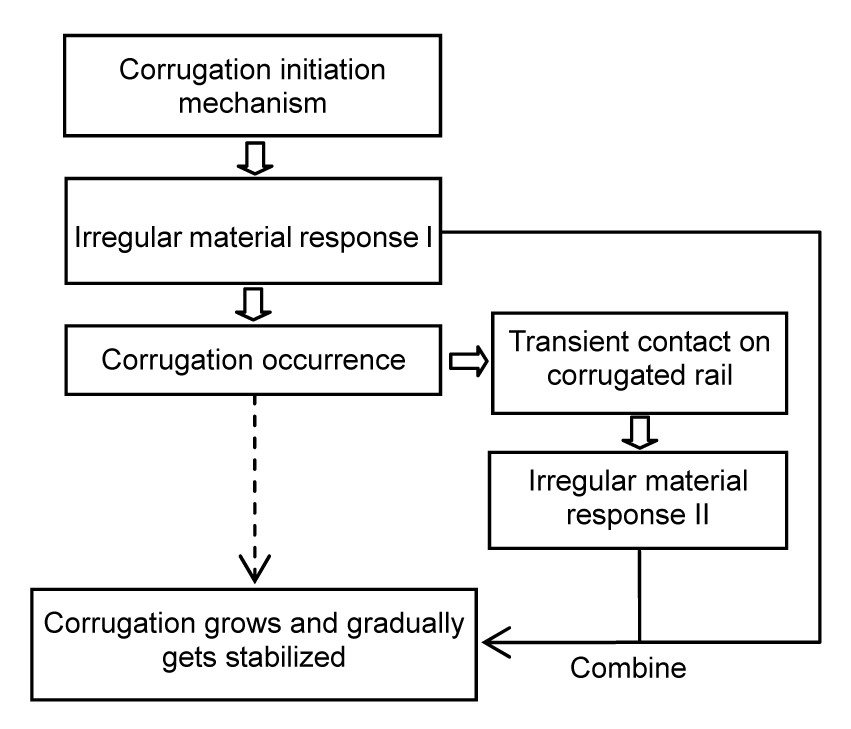
 The irregular material response caused by the initiation mechanism, hereinafter referred to as the irregular response I, should be larger at corrugation valleys and smaller at crests, i.e., leading to the occurrence of a corrugation. This is the dominant mechanism in the relatively early stages of a corrugation. Once the corrugation comes into being, another irregular material response also starts to act due to the geometric variation at the corrugation, referred hereinafter to as the irregular response II. The irregular response II is larger at crests than at valleys (Fig. 19), being very different from the irregular response I, especially at high speeds (smaller longitudinal shifts at higher speeds, Fig. 26a). Obviously, the irregular response II will alleviate the irregular response I due to their different patterns. Further considering that the irregular response II becomes more irregular with the corrugation depth (Fig. 23), at a certain depth the combined material response (irregular response I+II) starts to become regular, or the initiation mechanism and the consequence of the existing corrugation become balanced, i.e., the corrugation stabilizes. The phenomenon of corrugation stabilization has been observed in the field, e.g., the high-speed corrugations shown in Fig. 14b. Fig. 29 shows a schematic diagram to help understand the mechanism explained above. Note that other factors such as material work hardening and residual stresses could also play certain roles in the stabilization of corrugation.




 By changing the driving torque definition, braking cases can also be simulated by the 3D transient FE model, although only traction cases are presented in this paper due to space limitations. To authors’ experience, for the same friction exploitation level, the results of the braking and the traction cases indeed show some differences in contact stresses. In the future work, the 3D transient FE model can be employed to further study the material damage mechanisms on corrugated rails. Finally, it might be worthwhile to note that all discussions are mostly based on the numerical results shown above, in which influences of the lateral movement of the wheelset and the initiation mechanism of corrugation are not included.

6.  Summary and conclusions

 On the basis of field measurements and observations of (short-pitch) corrugations occurred on a recently opened Chinese high-speed line, a 3D transient rolling contact FE model is developed by an explicit FE approach to analyze the high-speed vehicle-track interaction in the presence of rail corrugations. The vehicle and the track subsystems are considered to ensure that the vehicle-track interaction is solved accurately in both the vertical and longitudinal directions. Detailed contact solutions on corrugated rails, including both the normal and the tangential solutions, are examined at different traction levels and at rolling speeds of up to 500 km/h. A summary of the results shown above and some conclusions are as follows.

1. The vertical and longitudinal (contact) forces, the pressure, and the surface shear stress all vary following the pattern of the corrugation, but with slightly different longitudinal phases. The patterns of the V-M stress and the frictional work are closer to that of the surface shear stress than to that of the pressure.

2. The discrete supports of the rail have considerable influences on the vehicle-track interaction on the corrugated rail at certain rolling speeds.

3. At certain friction exploitation levels, the state of rolling contact may oscillate between rolling-sliding and full sliding at the passing frequency of corrugation, leading to a significantly higher creepage than on smooth rails.

4. Fluctuation ranges of the V-M stress and the frictional work caused by a corrugation increase with the traction coefficient. This may explain why corrugation is more often observed on curves where the transmitted friction force is relatively high.

5. According to simulations by the nominal parameters, the wavelength of the corrugation occurring on the monitored Chinese high-speed line is most probably around 80 mm and a speed between 250 and 300 km/h is most detrimental, corresponding well to the corrugation shown in Fig. 1. Inevitable variations of the parameters along the track and their changes from the nominal values probably explain why the dominant corrugation wavelength found by CAT measurements is about 65 mm on sections where the running speed is about 300 km/h.

6. The traditional multi-body approach overestimates the dynamic wheel-rail interaction on corrugated rails, whereas results from the transient FE model should be more reasonable.

7. A theory is proposed to explain the observed phenomenon that the corrugation gradually stabilizes.

---

* Project supported by the National Natural Science Foundation of China (Nos. U1134202, 51275430, and 51305361), the National Basic Research Program (973) of China (No. 2011CB711103), and the Program for Changjiang Scholars and Innovative Research Team in University (Nos. IRT1178 and SWJTU12ZT01), China