Affiliation(s):
1. Department of Mathematics, University of Houston, Houston, Texas 77204-3008, USA; moreAffiliation(s): 1. Department of Mathematics, University of Houston, Houston, Texas 77204-3008, USA; 2. Department of Aerospace Engineering and Mechanics, University of Minnesota, Minnesota, MN 55455, USA; less
PAN Tsorng-Whay, GLOWINSKI Roland, JOSEPH Daniel D.. Simulating the dynamics of fluid-cylinder interactions[J]. Journal of Zhejiang University Science A, 2005, 6(2): 97-109.
@article{title="Simulating the dynamics of fluid-cylinder interactions", author="PAN Tsorng-Whay, GLOWINSKI Roland, JOSEPH Daniel D.", journal="Journal of Zhejiang University Science A", volume="6", number="2", pages="97-109", year="2005", publisher="Zhejiang University Press & Springer", doi="10.1631/jzus.2005.A0097" }
%0 Journal Article %T Simulating the dynamics of fluid-cylinder interactions %A PAN Tsorng-Whay %A GLOWINSKI Roland %A JOSEPH Daniel D. %J Journal of Zhejiang University SCIENCE A %V 6 %N 2 %P 97-109 %@ 1673-565X %D 2005 %I Zhejiang University Press & Springer %DOI 10.1631/jzus.2005.A0097
TY - JOUR T1 - Simulating the dynamics of fluid-cylinder interactions A1 - PAN Tsorng-Whay A1 - GLOWINSKI Roland A1 - JOSEPH Daniel D. J0 - Journal of Zhejiang University Science A VL - 6 IS - 2 SP - 97 EP - 109 %@ 1673-565X Y1 - 2005 PB - Zhejiang University Press & Springer ER - DOI - 10.1631/jzus.2005.A0097
Abstract: We present the simulation of the dynamics of fluid-cylinder interactions in a narrow three-dimensional channel filled with a Newtonian fluid, using a Lagrange multiplier based fictitious domain methodology combined with a finite element method and an operator splitting technique. As expected, a settling truncated cylinder turns its broadside perpendicular to the main stream direction and the center of mass moves to the central axis of the channel. In the case of two truncated cylinders, they first move around each other for a while and then stay together in a “T” shape. After the “T” shape has been formed for a long enough time, we found no vortex shedding behind the cylinders. When simulating the fluidization of 60 truncated cylinders, we captured the features of interactions among fluidized cylinders as observed in experiments.
Darkslateblue:Affiliate; Royal Blue:Author; Turquoise:Article
Article Content
. INTRODUCTION
The orientation of symmetric long bodies, e.g. ellipsoid and truncated cylinder, settling in liquids of different nature is a fundamental issue in many problems of practical interest (Liu and Joseph, 1993). In the past decade, a fast growing population of researchers developed numerical methods for direct simulation of fluid/particle interaction (Hu et al., 1992; Ladd, 1994a; 1994b; Qi and Luo, 2003; Hu, 1996; Johnson and Tezduyar, 1997; Maury and Glowinski, 1997; Hofler et al., 1998; Glowinski et al., 1999a; 2001; Takagi et al., 2003; Dong et al., 2004; Juárez et al., 2002). In this article we discuss first the generalization of a Lagrange multiplier based fictitious domain method (Glowinski et al., 1999a; 2001) for simulating the motion of particles with edges and corners, such as truncated cylinders, in a Newtonian fluid. Unlike the cases where the particles are spheres, we attach two points to each particle and move them according to the rigid-body motion of the particle. The equations describing the motion of these two points are solved by a distance preserving scheme so that rigidity can be maintained. Then we apply the above methodology to simulate the dynamics of fluid-cylinder interactions in a narrow three-dimensional channel filled with a Newtonian fluid. As expected, a settling truncated cylinder turns its broadside perpendicular to the main stream direction and the center of mass moves toward the central axis of the channel. In the case of two truncated cylinders, they first move around each other for a while after being released from their initial positions and then stay together in a “T” shape, as observed in experiments. We found that there is no vortex shedding behind the cylinders after the “T” shape has been formed for a long enough time. After increasing the density of the cylinders or reducing their length, we still obtained similar interaction between two settling truncated cylinders. In the simulation of fluidization of 60 truncated cylinders, we successfully captured the features of the interactions between fluidized cylinders as observed in experiments.
. A MODEL PROBLEM AND A FICTITIOUS DOMAIN FORMULATION FOR 3-D PARTICULATE FLOW
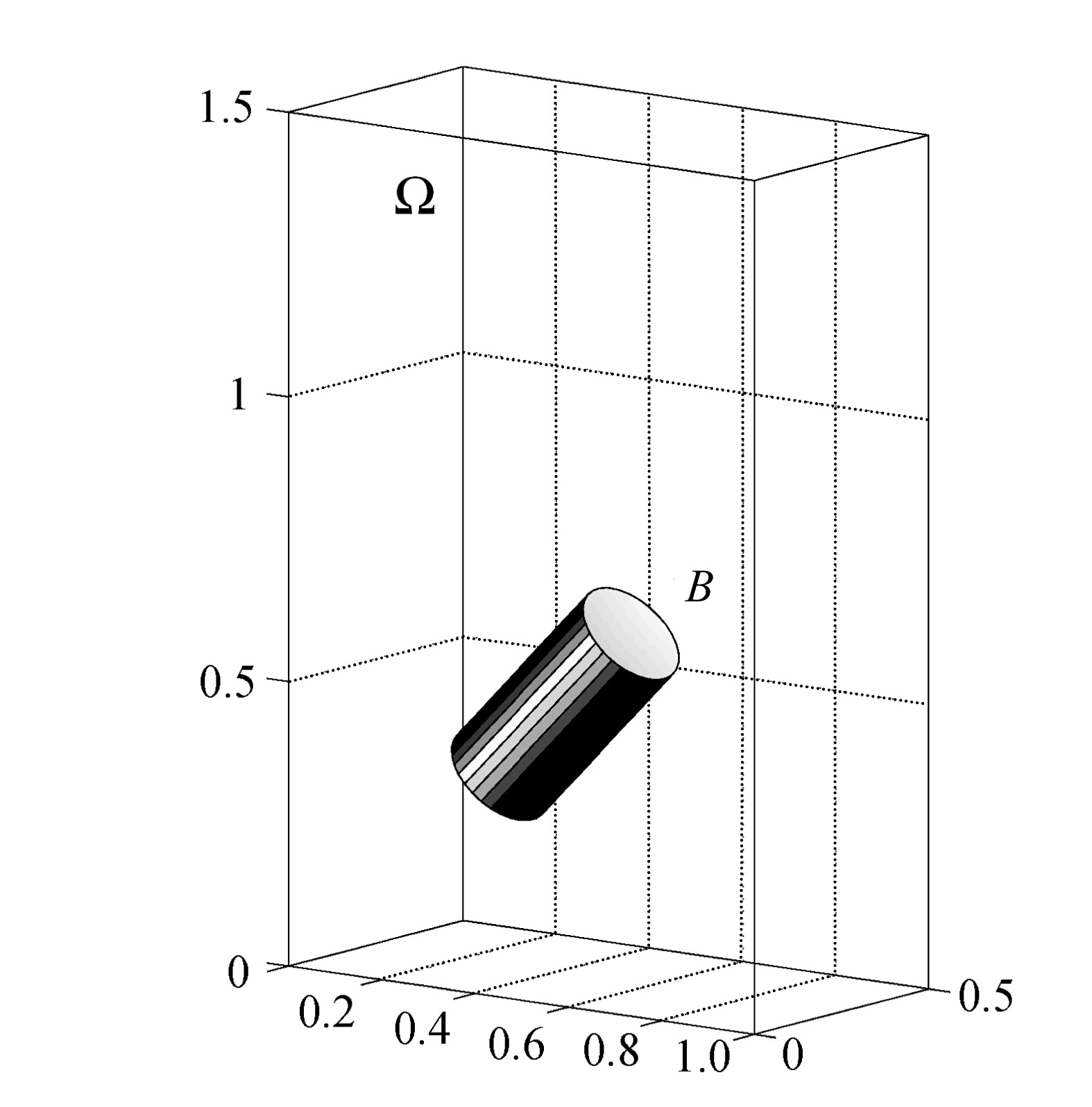
To perform the direct numerical simulation of the interaction between rigid bodies and fluids, we developed a methodology which combines a distributed Lagrange multiplier based fictitious domain (also called domain embedding) method with operator splitting methods (Glowinski et al., 1998b; 1999a; 1999b; 2001). In (Glowinski et al., 2001; Pan et al., 2001; 2002) we have applied this methodology to simulate the fluidization of a thousand spherical particles in 3-D and the sedimentation of ten thousand circular particles in 2-D. This approach (or closely related ones derived from it) has also been used by other investigators (Dong et al., 2004; Baaijens, 2001; Wagner et al., 2001; Yu et al., 2002; Diaz-Goano et al., 2003). We are going to recall the ideas at the basis of the above methodology by considering the motion of a single particle in a Newtonian viscous incompressible fluid (of density ρf and viscosity μf) under the effect of gravity. For the situation depicted in Fig.1 (a case where the particle has edges), the flow is modeled by the Navier-Stokes equations, namely, (with obvious notation) where Γ=∂Ω, g denotes gravity and n is the unit normal vector pointing outward to the flow region. We assume a no-slip condition on γ (=∂B). The motion of particle B satisfies the Euler-Newton’s equations, namely
Fig.1 The flow region with one cylinder
with the resultant and torque of the hydrodynamical forces given respectively by, with . Eqs.(1)−(7) are completed by the following initial conditions
and by the no-slip boundary conditions
Mp, Ip, G, V and ω above are the mass, inertia, center of mass, velocity of the center of mass and angular velocity of particle B, respectively. In Eq.(7) we found it preferable to deal with the kinematic angular momentum Ipω, thus making the formulation more conservative for non-spherical particle cases. To avoid particle-particle and particle-wall penetration which can happen in the numerical simulation, we introduced a artificial short-range repulsion force Fr in Eq.(6), which becomes active when the shortest distance between two (convex) particles or between (convex) particle and wall is less than a pre-chosen distance (Glowinski et al., 1999a; 2001; Maury, 1997) and then a torque in Eq.(7) acting on the point xr where Fr applies on B (see Remark 3 in Section 3.3 for the location of xr). For non-convex particles, we can apply similar approach to activate the short-range repulsion force Fr.
To solve system Eqs.(1)−(9) we can use, for example, Arbitrary Lagrange-Euler (ALE) methods as in ( Hu, 1996; Johnson and Tezduyar, 1997; Maury and Glowinski, 1997), or fictitious domain methods, which allow the flow calculation to be done on a fixed grid, as in (Glowinski et al., 1998b; 1999a; 1999b; 2001). The fictitious domain methods that we advocate have some common features with the immersed boundary method of Peskin (Peskin, 1977; 1981; Peskin and McQueen, 1980), but also some significant differences in the sense that we take advantage of distributed Lagrange multipliers to force the rigid body motion inside the particle. As with the methods in (Peskin, 1977; 1981; Peskin and McQueen, 1980), our approach takes advantage of the fact that the flow can be computed on a grid which does not have to vary in time, a substantial simplification indeed.
The principle of the fictitious domain method that we employ is rather simple. It consists in
(1) Filling the particles with a fluid having the same density and viscosity as the surrounding one.
(2) Compensating the above step by introducing, in some sense, an anti-particle of mass (−1)Mpρf /ρs and inertia (−1)Ipρf /ρs, taking into account the fact that any rigid body motion v(x, t) verifies ∇˙v=0 and D(v)=0 (ρs: particle density).
(3) Finally, assuming the fluid contained in B(t) has rigid body velocity,
via a Lagrange multiplier λ supported by . The vector λ forces rigidity in B(t) in the same way that ∇p forces ∇˙v=0 for incompressible fluids.
We obtain then an equivalent formulation of Eqs.(1)−(9) defined on the whole domain Ω, namely
For a.e. t>0, find {u(t), p(t), V(t), G(t), ω(t), λ(t)} such that
and
with the following functional spaces Various examples for in Eqs.(12) and (15) are given in (Glowinski et al., 2001; Glowinski, 2003). In Eqs.(11)−(17), only the center of mass, the translation velocity of the center of mass and the angular velocity of the particle are considered, which are sufficient for spherical particle cases. For non-spherical particles, knowing these two velocities and the center of mass of the particle, we can translate and rotate the particle in space by tracking, in each particle, two extra points x1 and x2 which follow the rigid body motion, namely
In practice we track two orthogonal normalized vectors rigidly attached to the body B and originating from the center of mass G.
Remark 1 The second gravity term on the right-hand-side of Eq.(12) can be combined with the pressure. Hence in the following discussion, this term will not be mentioned anymore.
. TIME AND SPACE DISCRETIZATION
. Lie’s first order operator-splitting scheme
Many operator-splitting schemes can be applied to problem (11)−(18). One advantage of operator-splitting schemes is that we can decouple difficulties such as (i) the incompressibility condition, (ii) the nonlinear advection term, and (iii) the rigid body motion, so that each one of them can be handled separately, and in principle optimally. Let Δt be a time discretization step and tn+s=(n+s)Δt. Application of Lie’s first order operator-splitting scheme (Chorin et al., 1978), to problem (11)−(18), yields:
for n≥0, un[u(tn)], Gn, Vn, ωn, and being known, we first compute un+1/6, pn+1/6 via the solution of
and set un+1/6=u(tn+1), pn+1/6=p(tn+1).
Next, compute un+2/6 via the solution of
and set un+2/6=u(tn+1).
Then, compute un+3/6 via the solution of
and set un+3/6=u(tn+1).
Now predict the motion of the center of mass and the angular velocity of the particle via the solution of
and set Gn+4/6=G(tn+1), Vn+4/6=V(tn+1), (Ipω)n+4/6=
(Ipω)(tn+1), and Using Gn+4/6, and obtained in the above step, we enforce the rigid body motion on the region Bn+4/6 occupied by the particle
and set un+1=u(tn+1), Vn+5/6=V(tn+1), (Ipω)n+5/6=
(Ipω)(tn+1).
Correct the motion of the center of mass and the angular velocity of the particle via the solution of
Then set Gn+1=G(tn+1), Vn+1=V(tn+1), (Ipω)n+1=
(Ipω)(tn+1), and In Eqs.(19)−(34), we have with Bn+4/6 being the region occupied by the particle B according to Gn+4/6, and and 0≤α,β≤1, with α+β=1. In numerical simulations, we always choose α=1 and β=0.
. Space discretization
We assume that and is a rectangular parallelepiped. For the finite element approximation of problem (11)−(18), we employ a Bercovier-Pironneau one, namely (Glowinski, 2003) where τh is a “tetrahedrization” of Ω, τ2h is twice coarser than τh, and P1 is the space of the polynomials in three variables of degree≤1. A finite dimensional space approximating Λ(t) is obtained as follows: let be a set of points from which cover (uniformly, for example); we define then where δ(˙) is the Dirac measure at x=0. Then we use <˙,˙>h defined by
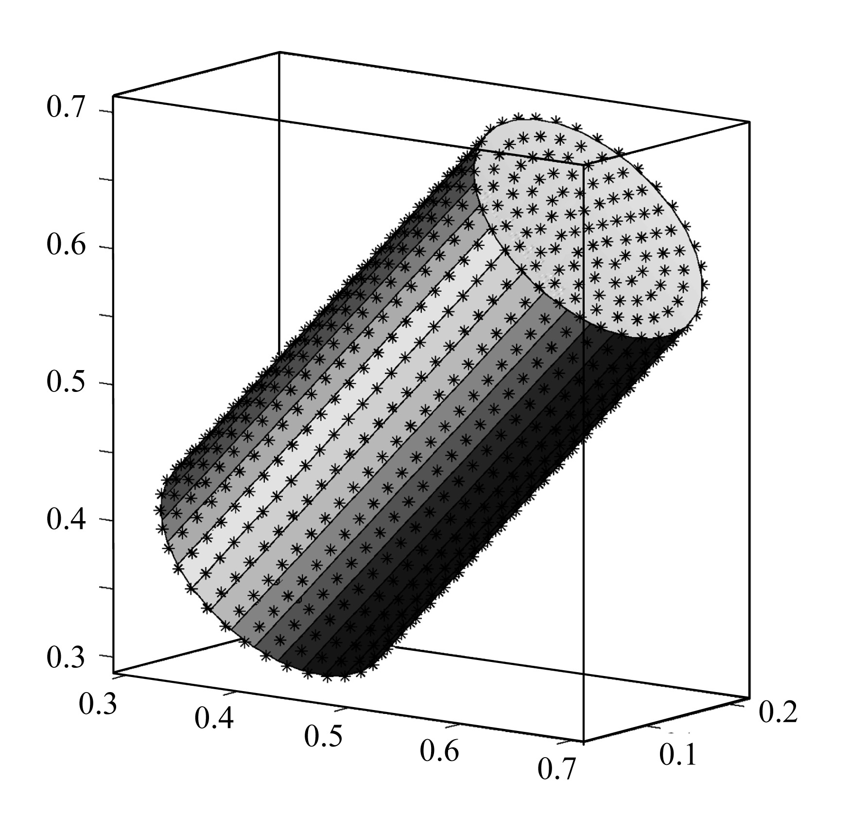
A typical choice of points for defining Eq.(38) is to take the grid points of the velocity mesh internal to the particle B and whose distance to the boundary of B is greater than, e.g. h/2, and to complete with selected points from the boundary of B(t) (see, e.g., Fig.2 for an example of selected collocation points on the boundary of B(t)).
Fig.2 An example of selected collocation points on the surface of a truncated cylinder
Using the above finite dimensional spaces and the backward Euler’s method for most of the subproblems in scheme (19)−(34), we obtain the following scheme after dropping some of the subscripts h [similar schemes are discussed in (Glowinski et al., 1998b; 1999a; 1999b; 2001)]:
For n≥0, un(u(tn)), Gn, Vn, ωn, and being known, we first compute un+1/6, pn+1/6 via the solution of
Next, compute un+2/6 via the solution of
and set un+2/6=u(tn+1). Then, compute un+3/6 via the solution of
Now predict the motion of the center of mass and the angular velocity of the particle via the solution of
G(tn) =Gn, V(tn) =Vn, (Ipω)(tn)=(Ipω)n, x1(tn)
Then set Gn+4/6=G(tn+1), Vn+4/6=V(tn+1), (Ipω)n+4/6 =(Ipω)(tn+1), and With Gn+4/6, and obtained at the above step, we enforce the rigid body motion on the region B(tn+4/6) occupied by the particle via the solution of
Correct the motion of the center of mass and the angular velocity of the particle via the solution of
Then set Gn+1=G(tn+1), Vn+1=V(tn+1), (Ipω)n+1=
(Ipω)(tn+1), and In Eqs.(40)−(55), <0} and = is an approximation of belonging to and verify Remark 2 The rate of convergence (with respect to h) of scheme (40)−(55), when using the Taylor-Hood finite element approximation instead of the Bercovier-Pironneau one, was investigated in (Juárez et al., 2002) for a circular particle in a Stokes flow, the error orders in the L2-norm for velocity and pressure slightly exceed 3 and 2, respectively.
. On the solution of subproblems (41), (42), (43), (44)−(48) and (49)−(50)
The degenerated quasi-Stokes problem (41) is solved by an Uzawa/preconditioned conjugate gradient algorithm as in (Glowinski et al., 1998b), where the discrete elliptic problems used for preconditioning are solved by a matrix-free fast solver from FISHPAK due to Adams et al.(1980). The stopping criterion for the preconditioned conjugate gradient algorithm is ||rk||/||r0||≤ε where rk is the residue at the kth iteration. It typically takes about 10 iterations in these simulations to achieve convergence when ε =10−5. The advection problem (42) for the velocity field is solved by a wave-like equation method as in (Dean and Glowinski, 1997; Dean et al., 1998). Problem (43) is a classical discrete elliptic problem which can be solved by the above matrix-free fast solver.
Systems (44)−(48) and (51)−(55) are systems of ordinary differential equations thanks to operator splitting. For their solutions one can choose a time step smaller than Δt, (i.e. we can divide Δt into smaller steps) to predict the translation velocity of the center of mass, the angular velocity of the particle, the position of the center of mass and the regions occupied by each particle so that the repulsion forces can effectively prevent particle-particle and particle-wall overlapping. At each sub-cycling time step, keeping the distance constant between points x1 and x2 in each particle is important since we are dealing with rigid particles. To satisfy the above constraint we applied the following approach:
1. Translate x1 and x2 according to the new position of the mass center at each subcycling time step; 2. Rotate Gx1 and Gx2, the relative positions of x1 and x2 to the center of mass G, by the following Crank-Nicolson scheme (a Runge-Kutta scheme of order 2, in fact):
for i=1, 2 with τ as a sub-cycling time step. By Eq.(56), we have , for i=1, 2 and (i.e., scheme (56) is distance and in fact shape preserving).
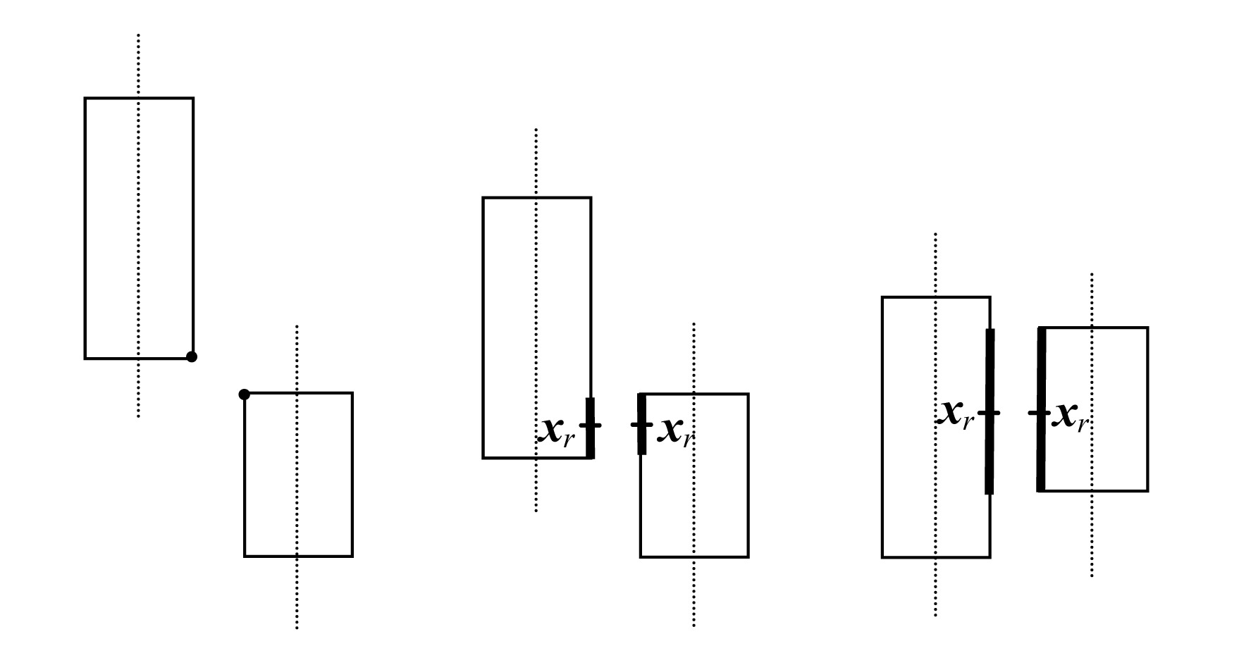
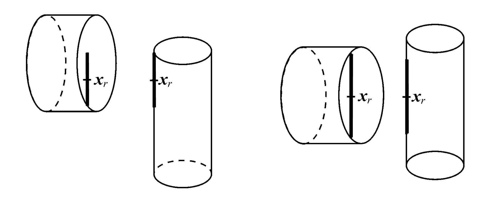
Remark 3 In order to activate the short range repulsion force in Eqs.(6) and (7), we have to find the shortest distance between two truncated cylinders. Unlike the cases for spheres, it is not trivial to locate the points on the surface of each truncated cylinder so that their distance is the shortest possible between two truncated cylinders. There is no explicit formula for such distance. The difficulties stem from the fact that a truncated cylinder is not a strictly convex set; it is “flat” in the direction of the central axis and on the disks at the two ends. When two cylinders are parallel to each other, i.e., when the two central axes are parallel to each other, the question which arises is: at which points do we have to apply the repulsion force when it is needed As shown in Fig.3, the shortest distance is between two line segments on the cylinder surfaces on the plane passing through two central axes. We choose the middle point on each line segment as the point at which we apply the repulsion force as shown in Fig.3. When the plane containing one end disk is parallel to the central axis of another cylinder, e.g., two cylinders are in a “T” shape as in Fig.4, we also first obtain the line segment from the circular surface of one cylinder and that from the disk at one end of another cylinder so that the shortest distance is between two line segments. Then we choose the middle point on each line segment as the point at which we apply the repulsion force. When the cylinders are not parallel to each other, we first choose a set of points from the surface of each truncated cylinder. Then we find the point among the chosen points from each surface at which the distance is the shortest. We repeat this (kind of relaxation) process in the neighborhood of the newly located point on each surface of the cylinder until convergence, usually obtained in very few iterations. For the shortest distance between the wall and truncated cylinder, we can take the advantage of the shape of truncated cylinder and only search points on the circles at the two ends and then determine the shortest distance to each wall and whether it is parallel to the wall. When it is parallel to the wall then we use the midpoint on the line segment, which is either parallel to the central axis and on the surface or on the plane containing the disk at the end, as the point for applying the repulsion force. These technical details have to be implemented in order to capture the interactions between cylinders.
Fig.3 Possible relative positions of two parallel cylinders on the plane passing through two central axes: (a) the shortest distance is between two corner points (left pair), (b) the distance between two thicker line segments is the shortest (middle and right pairs)
Fig.4 Possible relative positions of two cylinders forming “T” shape: the distance between two thicker line segments is the shortest
The rigid body motion is enforced in B(tn+4/6), via Eq.(50). At the same time those hydrodynamical and gravity forces acting on the particles are also taken into account in order to update the translation and angular velocities of the particles. To solve Eqs.(49)−(50), we use a conjugate gradient algorithm as discussed in (Glowinski et al., 1999a). Since we take β=0 in Eq.(49) for the simulation, we actually do not need to solve any non-trivial linear systems for the velocity field; this saves a lot of computing time. To get the angular velocity ωn+1, computed via
We need to have , the inertia of the particle B(tn+4/6). We first compute the inertia I0 in the coordinate system attached to the particle. Then via the center of mass Gn+4/6 and points and , we have the rotation transformation Q (QQT=QTQ=Id, detQ=1) which transforms vectors expressed in the particle frame to vectors in the flow domain coordinate system and . Actually in order to update matrix Q we can also use quaternion techniques, as shown, in the review paper (Chou, 1992).
. NUMERICAL EXPERIMENTS
. Settling of a truncated cylinder in a 2D-like channel
In the first test case, we consider the simulation of the motion of a truncated cylinder settling in an infinite length narrow channel filled with a Newtonian fluid. The computational domain is Ω=(0, 1)×(0, 0.25)×(0, 4) initially, then it moves down with the mass center of the cylinder (see, e.g., (Hu et al., 1992) for adjusting the computational domain according to the position of the particle). The fluid density is ρf=1 and the fluid viscosity is μf=0.01. The flow field initial condition is u=0. The density of the cylinder is ρs= 1.1. The radius of the cylinder is 0.1 and its length is 0.4. Initially its central axis is in the vertical direction. The initial position of the mass center is at (0.5, 0.125, 1). The initial translation and angular velocities of the cylinder are 0. To check the convergence, we chose the following two pairs of the mesh size of the velocity field and the time step: {hv, Δt}={1/80, 0.001}, {1/112, 0.001}. The mesh size of the pressure is always hp=2hv.
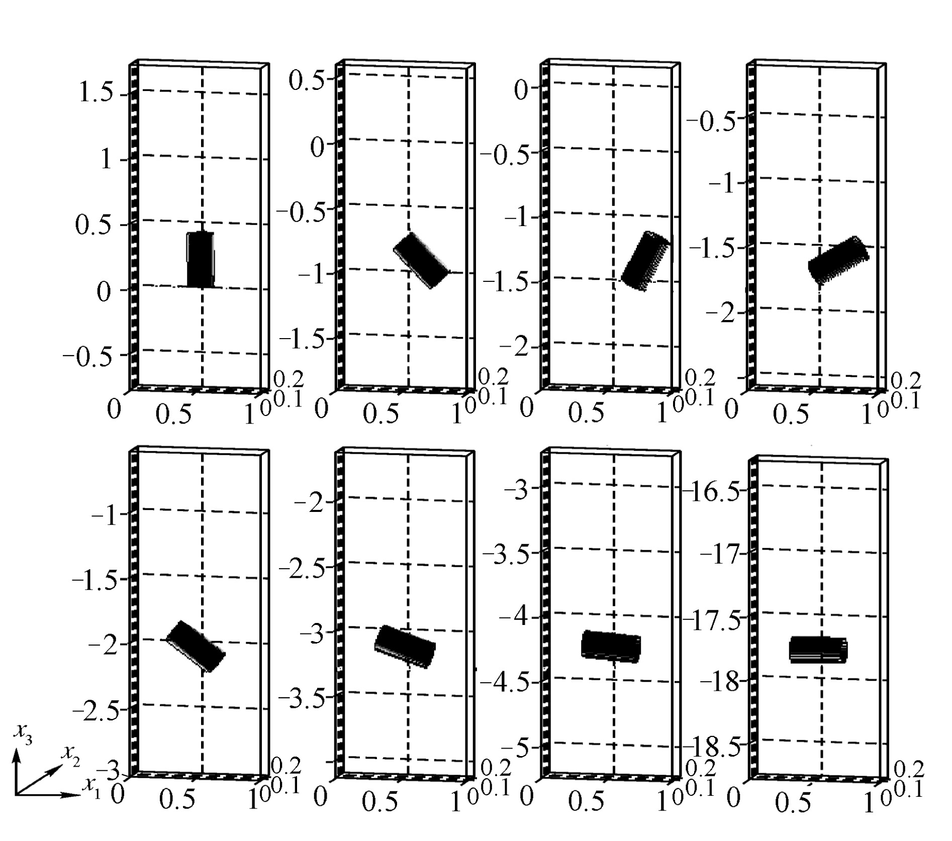
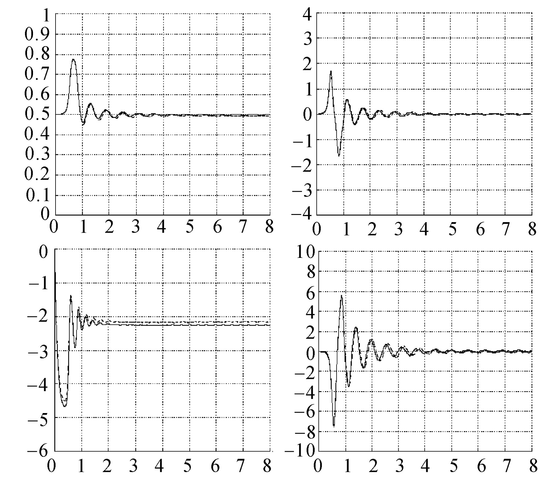
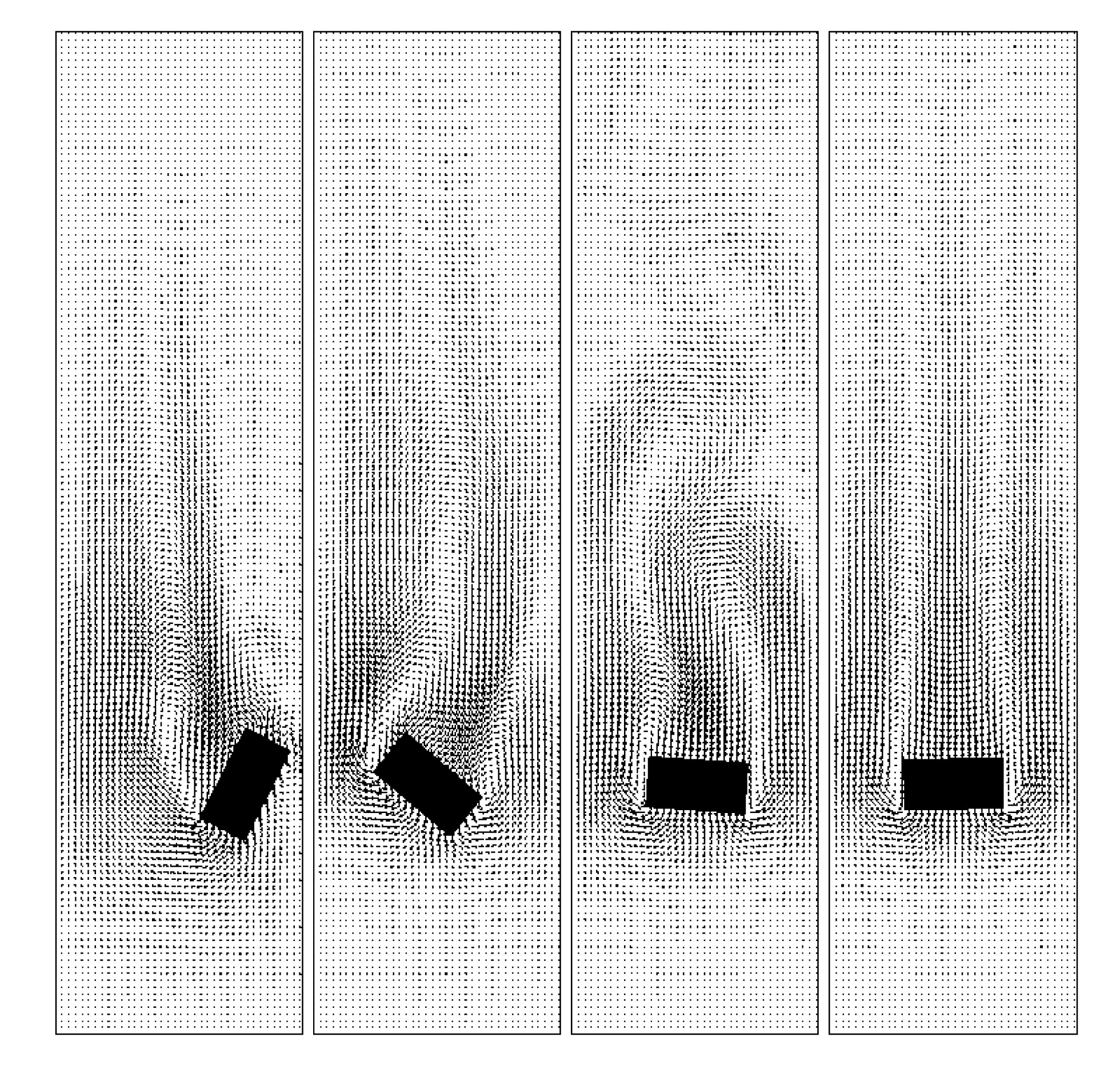
The snapshots of the cylinder position and its orientation for {hv, Δt}={1/112, 0.001} at different times in the channel are shown in Fig.5. The computations were performed in a moving frame of reference, so the cylinder does not appear moving downward. In Fig.6 we show the histories versus time of the x1-coordinate of the mass center, the x1- and x3-components of the translation velocity and the x2-component of the angular velocity. We obtained a good agreement between these results. The movement of the cylinder is very fast at the beginning when it moves toward the side wall after being released from its initial position. Later on the oscillations were damped out (Fig.6). As expected, the truncated cylinder turns its broadside perpendicular to the main stream direction and the mass center moves back to the central axis of the channel. The velocity fields projected on the x1x3-plane passing through the mass center are shown in Fig.7 for hv=1/112 and Δt=0.001.
Fig.5 Position and orientation of the cylinder at t=0.25, 0.5, 0.7, 0.8, 1, 1.5, 2 and 8 (from left to right and from top to bottom)
Fig.6 Histories of the x1-coordinate of the mass center (upper left), of the x1-component of the velocity of the mass center (upper right), of the x3-component of the velocity of the mass center (lower left), and of the x2-component of the angular velocity (lower right) (hv=1/80 and Δt=0.001, dashed lines; hv=1/112 and Δt=0.001, solid lines)
Fig.7 Velocity field at t=0.7, 1, 2 and 8 on the x1x3-plane passing through the mass center of the cylinder (from left to right)
For hv=1/112 and Δt=0.001, the averaged particle velocity when the cylinder reaches a stable position is about 2.255 (the maximal velocity is about 4.681) so the averaged particle Reynolds number with the longest axis as characteristic length is 90.2. The number of nodes for the velocity field is 546021 (resp., 1471373) for hv=1/80 (resp., 1/112). The memory used in the simulation is about 69 MB (resp., 184 MB) for hv=1/80 (resp., 1/112). The simulation takes about 14 s (resp., 38 s) per time step for {hv, Δt}={1/80, 0.001} (resp., {1/112, 0.001}) on a Linux based PC with 1.6 GHz AMD Athlon CPU.
. Two truncated cylinder settling in a 2D-like channel
Fig.10.4.9 in (Joseph, 1992) shows experimental results; we can observe many types of interactions among truncated cylinders when fluidized in a 2D-like bed (there is only one layer of particles in a narrow channel). Even though they are fluidized, the features of interaction between two truncated cylinders are similar to those of two truncated cylinders settling in a 2D-like channel. To reproduce some of those features computationally, we consider the following test case. The initial mass center positions are (0.45, 0.125, 1) and (0.45, 0.125, 1.3), respectively. The central axes are in the horizontal direction initially so the frames rigidly attached to the cylinders are {(1, 0, 0), (0, 1, 0), (0, 0, 1)} initially. The radii are 0.1 and their lengths are 0.46; we have taken {1/80, 0.001} and {1/112, 0.001} for {hv, Δt}. All other parameters are as in the previous case.
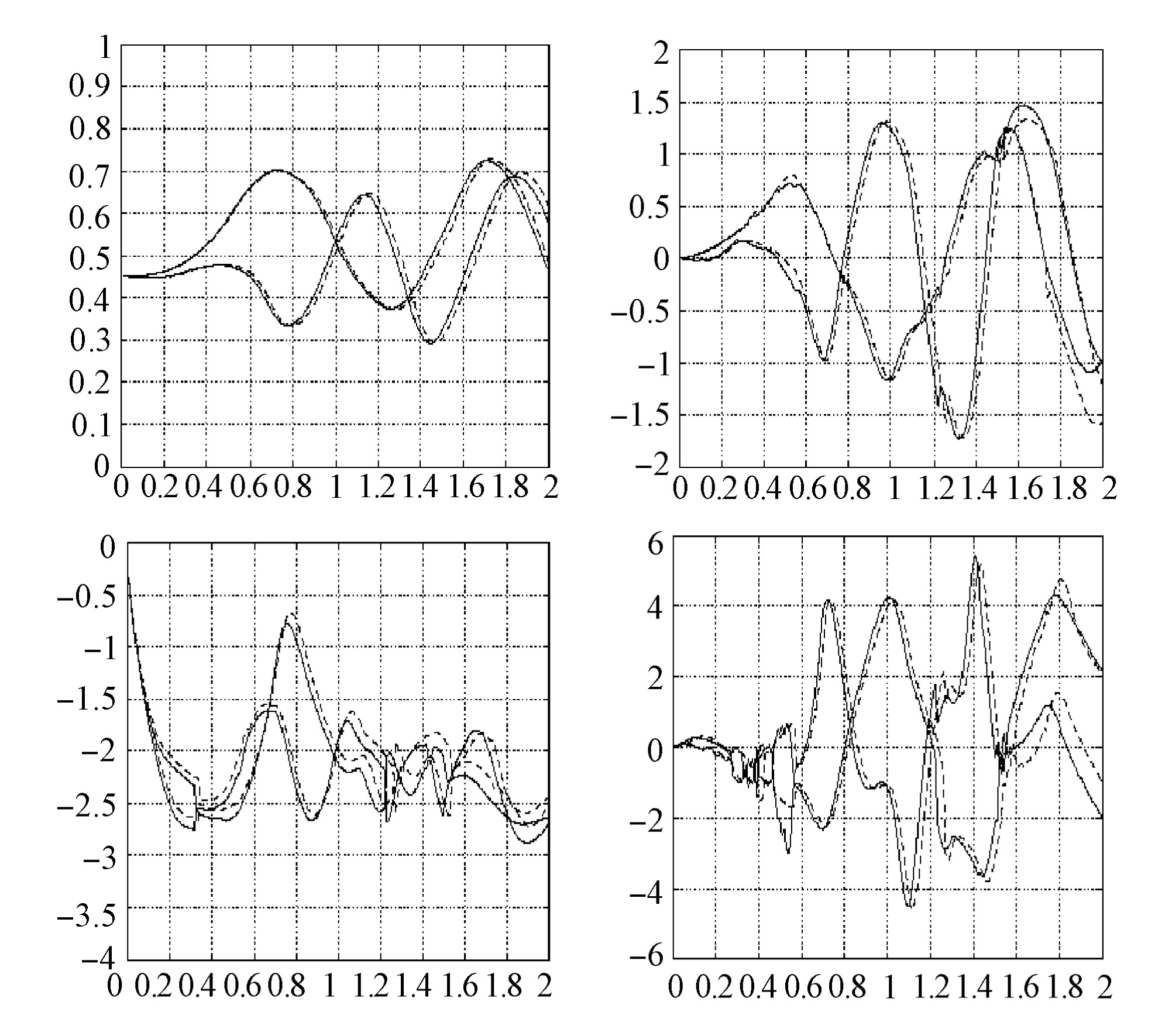
Fig.10 Histories of the x1-coordinate of the mass center (upper left), the x1-component of the translation velocity of the mass center (upper right), the x3-component of the translation velocity of the mass center (lower left), and the x2-component of the angular velocity (lower right) (hv=1/80 and Δt=0.001, dashed lines; hv=1/112 and Δt=0.001, solid lines)
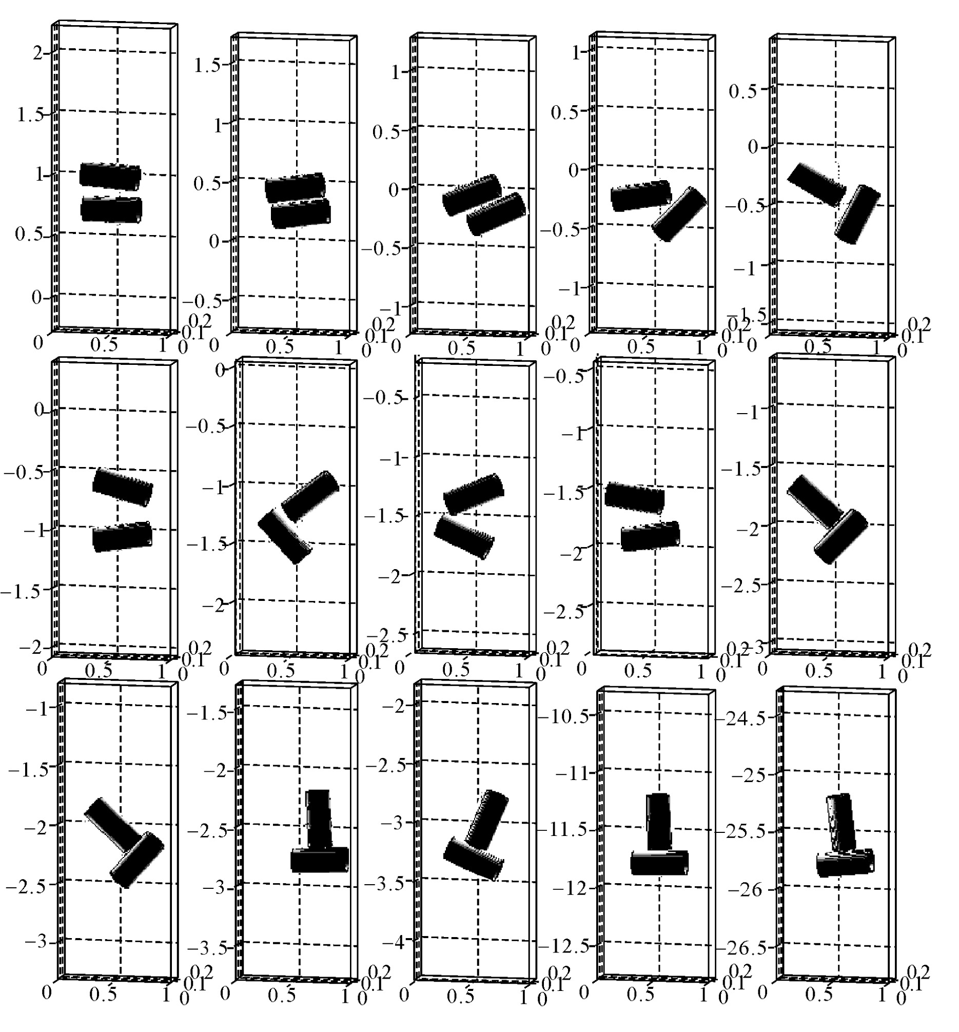
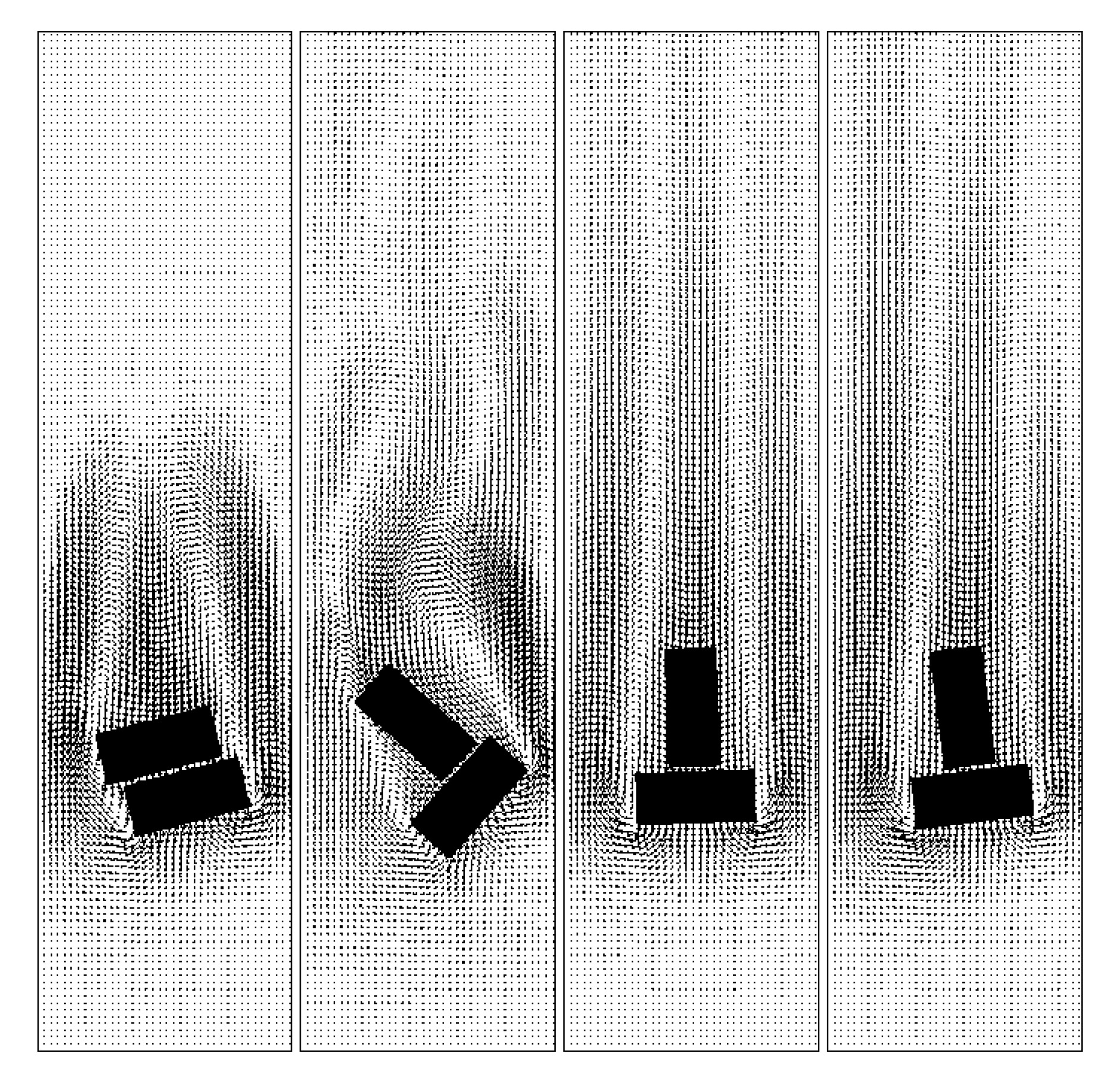
Snapshots of the positions and orientations of two cylinders for {hv, Δt}={1/112, 0.001} are shown in Fig.8. The cylinders first move around each other and then stay together in a “T” shape, as had been observed in experiments. Snapshots of the velocity field for {hv, Δt}={1/112, 0.001} projected on the x1x3-plane passing through the mass center of the upper cylinder are shown in Fig.9. As observed in the experiments shown in (Joseph, 1992), we observed that in Fig.9 the wake behind the lower cylinder makes it and the other cylinder stay together to form a “T” shape configuration. We also observed that there is no vortex shedding behind the cylinders after the “T” shape configuration has been formed for a sufficiently long time (see snapshots at t=5 and 10). For {hv, Δt}={1/80, 0.001} and {1/112, 0.001}, the histories of the x1-coordinates, the x1- and x3-components of the translation velocities of the mass center, and the x2-component of the angular velocities are shown in Fig.10 for 0≤t≤2. We obtained a good agreement between results, considering the violence of the motion during the first two time units. For the last two time units (8≤t≤10), the averaged particle speed is 2.794 so that the averaged particle Reynolds number with the cylinder length as characteristic length is 128.524. The maximal averaged speed of the two cylinders is 2.971 for 0≤t≤10.
Fig.8 Position and orientation of two cylinders at t=0.2, 0.5, 0.6, 0.7, 0.8, 1, 1.2, 1.3, 1.4, 1.5, 1.6, 1.8, 2, 5 and 10 (from left to right and from top to bottom)
Fig.9 Velocity field at t=0.5, 1.6, 5 and 10 on the x1x3-plane passing through the mass center of the upper cylinder for {hv, Δt}={1/112, 0.001} (from left to right)
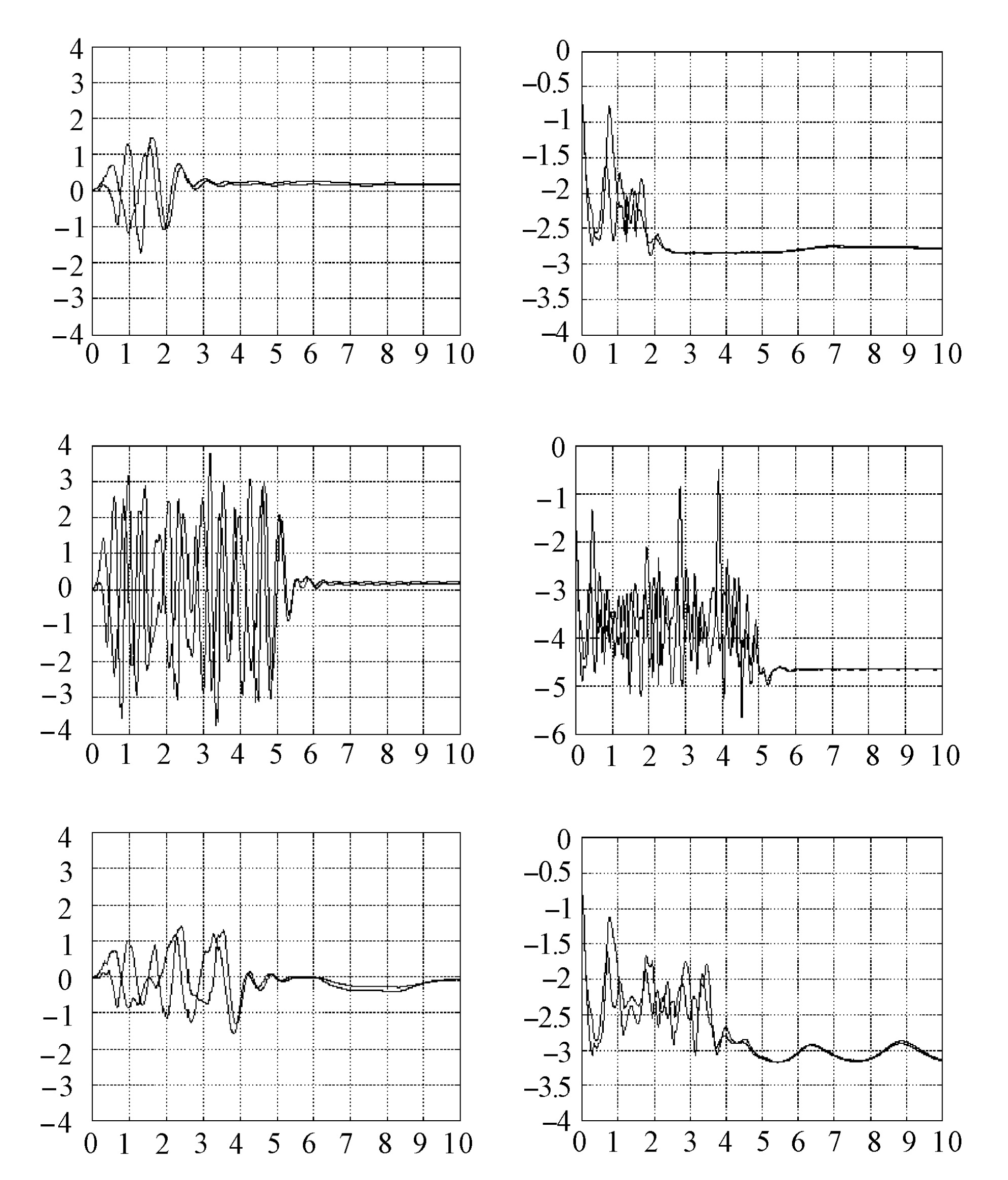
To see the effect of the length and the density of the cylinder, we considered the two following tests. We only either increase the density of cylinders to 1.25 or reduce the lengths to 0.4 and keep all other parameters the same as above with {hv, Δt}={1/112, 0.001}. The numerical results of both cases are similar to those of the above case. Histories of the translation velocity of the mass center are shown in Fig.11.
Fig.11 Histories of the x1-component (upper left) and the x3-component (upper right) of the translation velocity of the mass center for the first test case, those of the test case of density 1.25 (middle left and middle right), and those of the test case of length 0.4 (lower left and lower right) considered in Section 4.2
The memory used in the simulation was about 71 MB (resp., 190 MB) for hv=1/80 (resp., 1/112) for the first test case. The simulation takes about 5.76 s (resp., 14.34 s) per time step for {hv, Δt}={1/80, 0.001} (resp., {1/112, 0.001}) on a Linux based PC with 2.2 GHz Opteron 248 CPU.
. Fluidization of 60 truncated cylinders in a 2D-like channel
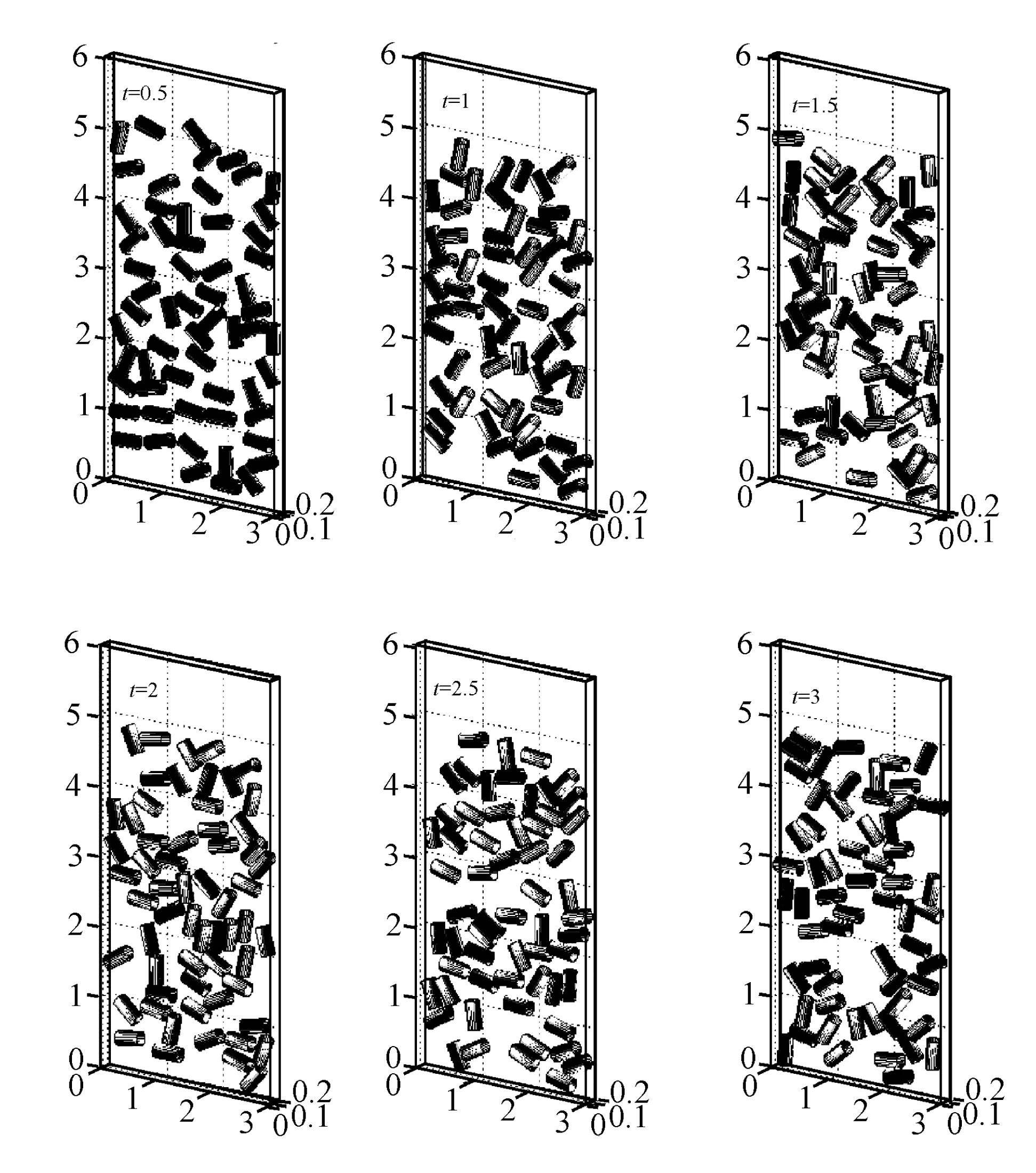
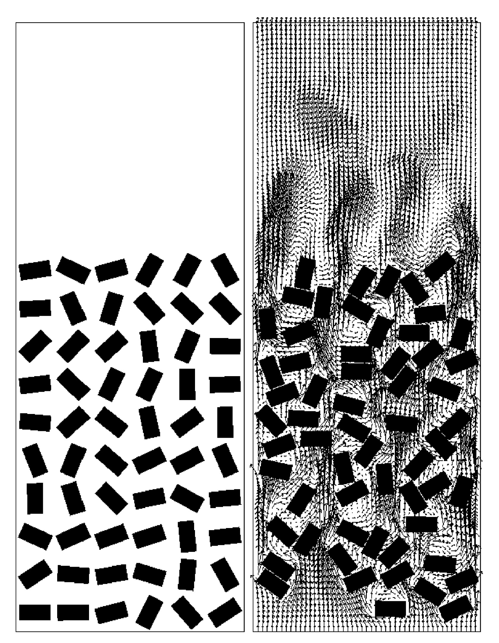
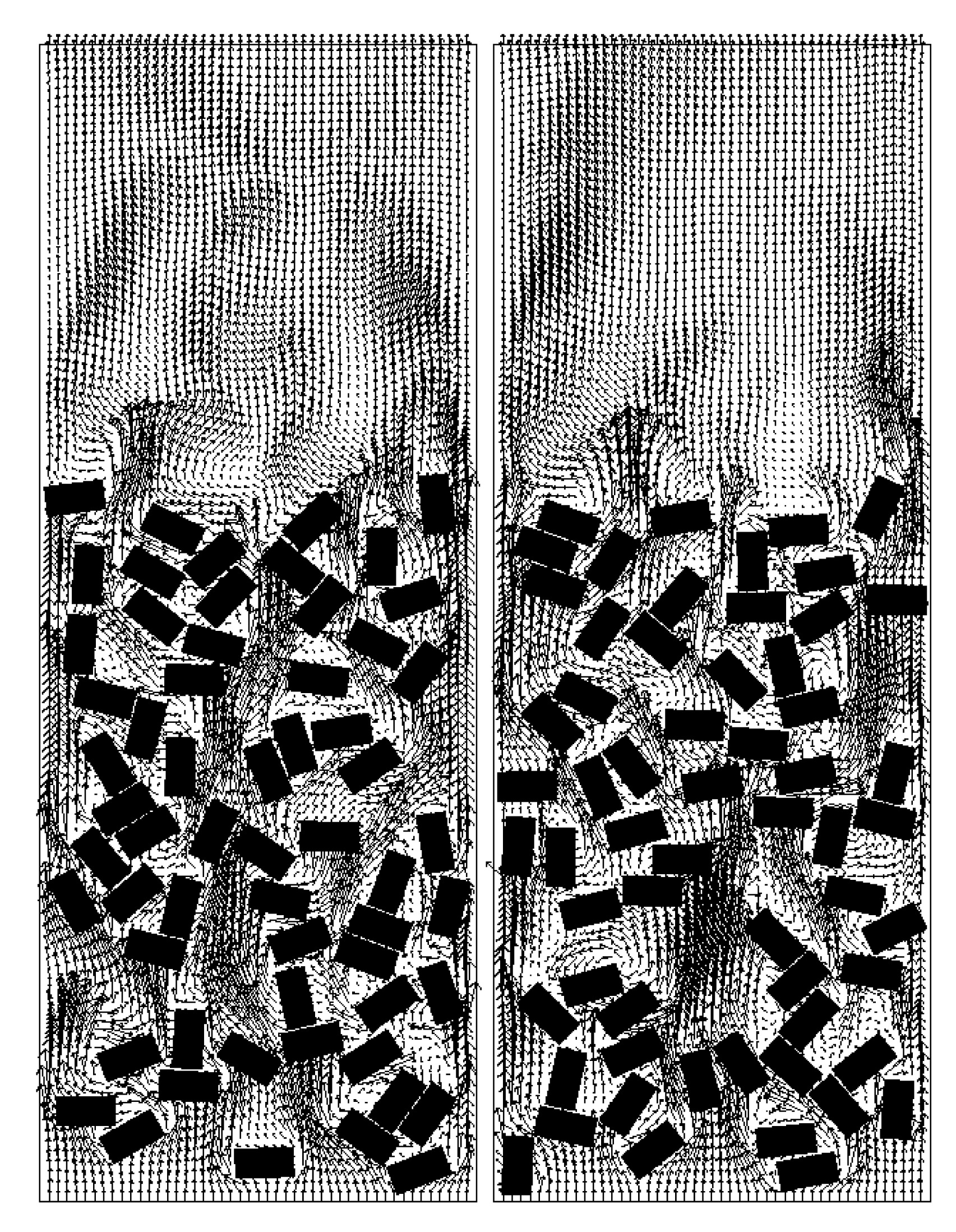
To simulate the fluidization of truncated cylinders similar to the one shown in Fig.10.4.9 in (Joseph, 1992), we considered the following test case. The computational domain is Ω=(0, 3)×(0, 0.25)×(0, 8). The initial mass center positions and orientations are shown in Fig.13 with randomly chosen angle. The radii are 0.1, their lengths are 0.4 and {hv, Δt}={1/80, 0.001}. All other parameters are as in the case in Section 4.1. At the bottom and the top of the channel, the velocity field is (0, 0, U(t)) with U(t)=1.5(1−e−20t). In Figs.12, 13 and 14 the snapshots of the position and orientation of the cylinders and the velocity fields projected to the x1x3 central plane are shown. We successfully captured the features shown in Fig.10.4.9 in (Joseph, 1992). For 0≤t≤3 the averaged speed of particles is 1.109 and the maximal averaged speed of 60 cylinders is 1.476. But for a single cylinder, the maximal speed is 4.931 for 0≤t≤3. Hence the particle Reynolds numbers based on the length of the cylinders are 44.36, 59.04 and 197.24, respectively. The memory used in the simulation was about 507 MB and it takes about 103.13 s per time step on a Linux-based PC with 2.2 GHz Opteron 248 CPU.
Fig.12 Position of the cylinders at t=0.5, 1, 1.5, 2, 2.5 and 3 (from left to right and from top to bottom)
Fig.13 Velocity field at t=0 and 1 on the x1x3 central plane (from left to right)
Fig.14 Velocity field at t=1.5 and 3.0 on the x1x3 central plane (from left to right)
Acknowledgements
We acknowledge the helpful comments and suggestions of R. Bai, E.J. Dean, J. He, H.H. Hu, P.Y. Huang, G.P. Galdi, Y. Kuznetsov and J. Periaux.
[1] Adams, J., Swarztrauber, P., Sweet, R., 1980. FISHPAK: A Package of Fortran Subprograms for the Solution of Separable Elliptic Partial Differential Equations. , The National Center for Atmospheric Research, Boulder, CO, :
[2] Baaijens, F.P.T., 2001. A fictitious domain/mortar element method for fluid structure interaction. Int J Numer Meth Fluids, 35:743-761.
[3] Chorin, A.J., Hughes, T.J.R., Marsden, J.E., McCracken, M., 1978. Product formulas and numerical algorithms. Comm Pure Appl Math, 31:205-256.
[4] Chou, J.C.K., 1992. Quaternion kinematic and dynamic differential equations. IEEE Transaction on Robotics and Automation, 8:53-64.
[5] Dean, E.J., Glowinski, R., 1997. A wave equation approach to the numerical solution of the Navier-Stokes equations for incompressible viscous flow. C R Acad Sc Paris, 325(Srie 1):783-791.
[6] Dean, E.J., Glowinski, R., Pan, T.W., 1998. A Wave Equation Approach to the Numerical Simulation of Incompressible Viscous Fluid Flow Modeled by the Navier-Stokes Equations. De Santo, J.A, (Ed.), Mathematical and Numerical Aspects of Wave Propagation. SIAM, Philadelphia,:65-74.
[7] Diaz-Goano, C., Minev, P.D., Nandakumar, K., 2003. A fictitious domain/finite element method for particulate flows. J Comp Phy, 192:105-123.
[8] Dong, S., Liu, D., Maxey, M., Karniadakis, G.E., 2004. Spectral distributed multiplier (DLM) method: Algorithm and benchmark test. J Comp Phys, 195:695-717.
[9] Glowinski, R., 2003. Finite Element Methods for the Numerical Simulation of Unsteady Incompressible Viscous Flow Modeled by the Navier-Stokes Equations. Handbook of Numerical Analysis, Vol, IX. North-Holland, Amsterdam,:1-1176.
[10] Glowinski, R., Pan, T.W., Hesla, T., 1998. A Fictitious Domain Method with Distributed Lagrange Multipliers for the Numerical Simulation of Particulate Flow. Domain Decomposition Methods 10, American Mathematical Society, Providence,:121-137.
[11] Glowinski, R., Pan, T.W., Periaux, J., 1998. Distributed Lagrange multiplier methods for incompressible flow around moving rigid bodies. Comput Methods Appl Mech Engrg, 151:181-194.
[12] Glowinski, R., Pan, T.W., Hesla, T., Joseph, D.D., 1999. A distributed Lagrange multiplier/fictitious domain method for flows around moving rigid bodies: Application to particulate flows. Int J Multiphase Flow, 25:755-794.
[13] Glowinski, R., Pan, T.W., Hesla, T., Joseph, D.D., Priaux, J., 1999. A distributed Lagrange multiplier/fictitious domain method for flow around moving rigid bodies: Application to particulate flow. Int J Num Meth in Fluids, 30:1043-1066.
[14] Glowinski, R., Pan, T.W., Hesla, T., Joseph, D.D., Priaux, J., 2001. A fictitious domain approach to the direct numerical simulation of incompressible viscous flow past moving rigid bodies: Application to particulate flow. J Comput Phys, 169:363-426.
[15] Hofler, K., Muller, M., Schwarzer, S., 1998. Interacting Particle-Liquid Systems. High Performance Computing in Science and Engineering, Springer-Verlag, Berlin,:54-64.
[16] Hu, H.H., 1996. Direct simulation of flows of solid-liquid mixtures. Int J Multiphase Flow, 22:335-352.
[17] Hu, H.H., Joseph, D.D., Crochet, M.J., 1992. Direct simulation of fluid particle motions. Theoret Comput Fluid Dynamics, 3:285-306.
[19] Johnson, A., Tezduyar, T., 1997. 3-D simulation of fluid-rigid body interactions with the number of rigid bodies reaching 100. Comp Meth Appl Mech Eng, 145:301-321.
[20] Jurez, L.H., Glowinski, R., Pan, T.W., 2002. Numerical simulation of the sedimentation of rigid bodies in an incompressible viscous fluid by Lagrange multiplier/fictitious domain methods combined with the Taylor-Hood finite element approximation. J Scientific Computing, 17:683-694.
[21] Ladd, A.J.C., 1994. Numerical simulations of particulate suspensions via a discretized Boltzmann equation, Part 1, Theoretical foundation. J Fluid Mech, 271:285-310.
[22] Ladd, A.J.C., 1994. Numerical simulations of particulate suspensions via a discretized Boltzmann equation, Part 2, Numerical results. J Fluid Mech, 271:311-340.
[23] Liu, Y.J., Joseph, D.D., 1993. Sedimentation of particles in polymer solutions. J Fluid Mech, 255:565-595.
[24] Marchuk, G.I., 1990. Splitting and Alternating Direction Methods. Handbook of Numerical Analysis, Vol, I. North-Holland, Amsterdam,:197-462.
[25] Maury, B., Glowinski, R., 1997. Fluid-particle flow: a symmetric formulation. C R Acad Sc Paris, 324(Srie 1):1079-1084.
[26] Maury, B., 1997. A many-body lubrication model. C R Acad Sc Paris, 325(Srie 1):1053-1058.
[27] Pan, T.W., Joseph, D.D., Glowinski, R., 2001. Modeling Rayleigh-Taylor instability of a sedimenting suspension of several thousand circular particles in a direct numerical simulation. J Fluid Mech, 434:23-37.
[28] Pan, T.W., Joseph, D.D., Bai, R., Glowinski, R., Sarin, V., 2002. Fluidization of 1204 spheres: simulation and experiments. J Fluid Mech, 451:169-191.
[29] Peskin, C.S., 1977. Numerical analysis of blood flow in the heart. J Comp Phys, 25:220-252.
[30] Peskin, C.S., 1981. Lectures on mathematical aspects of physiology. Lectures in Applied Math, 19:69-107.
[31] Peskin, C.S., McQueen, D.M., 1980. Modeling prosthetic heart valves for numerical analysis of blood flow in the heart. J Comp Phys, 37:113-132.
[32] Qi, D., Luo, L.S., 2003. Rotational and orientational behaviour of three-dimensional spheroidal particles in Couette flows. J Fluid Mech, 477:201-213.
[33] Takagi, S., Oguz, H.N., Zhang, Z., Prosperetti, A., 2003. PHYSALIS: A new method for particle simulation. Part II: Two-dimensional Navier-Stokes flow around cylinders. J Comput Phys, 187:371-390.
[34] Wagner, G.J., Moes, N., Liu, W.K., Belytschko, T., 2001. The extended finite element method for rigid particles in Stokes flow. Int J Numer Meth Engng, 51:293-313.
[35] Yu, Z., Phan-Thien, N., Fan, Y., Tanner, R.I., 2002. Viscoelastic mobility problem of a system of particles. J Non-Newtonian Fluid Mech, 104:87-124.
Open peer comments: Debate/Discuss/Question/Opinion

Open peer comments: Debate/Discuss/Question/Opinion
<1>