Similar articles

Abstract: In this paper, a prediction model is developed that combines a gaussian mixture model (GMM) and a kalman filter for online forecasting of traffic safety on expressways. Raw time-to-collision (TTC) samples are divided into two categories: those representing vehicles in risky situations and those in safe situations. Then, the GMM is used to model the bimodal distribution of the TTC samples, and the maximum likelihood (ML) estimation parameters of the TTC distribution are obtained using the expectation-maximization (EM) algorithm. We propose a new traffic safety indicator, named the proportion of exposure to traffic conflicts (PETTC), for assessing the risk and predicting the safety of expressway traffic. A kalman filter is applied to forecast the short-term safety indicator, PETTC, and solves the online safety prediction problem. A dataset collected from four different expressway locations is used for performance estimation. The test results demonstrate the precision and robustness of the prediction model under different traffic conditions and using different datasets. These results could help decision-makers to improve their online traffic safety forecasting and enable the optimal operation of expressway traffic management systems.

1.  Introduction

 Road traffic accidents are one of the world’s largest public health and injury problems. According to the World Health Organization (WHO), more than a million people are killed on the world’s roads each year. Thus, the measurement, assessment and forecasting of traffic safety are very important topics that may be applied in transportation planning, operation, and management (Meng et al., 2011a; 2011b). Traffic safety is most commonly measured in terms of the number of traffic accidents and the consequences of those accidents in terms of fatalities and injuries of differing severities (Qu et al., 2011). This is generally regarded as a reactive rather than a proactive approach in that it is based on the collection and analysis of accident data by the police and other authorities after the accidents have actually happened. Because accidents occur randomly in time and space, traffic safety is a particularly difficult phenomenon to study, thereby making its measurement, assessment and comparison difficult as well (Archer, 2004). For traffic planning purposes, levels of traffic safety for a given traffic site may be predicted based on long-term historical accident data. However, for the purposes of traffic management, short-term traffic safety forecasting is very limited by the coverage, quality and usefulness of the accident data. Thus, the underlying principle for a more effective short-term traffic safety evaluation strategy is to develop proximal safety indicators that represent the temporal and spatial proximity characteristics of unsafe interactions and near-accidents.

 These “safety indicators” are usually defined as traffic measures that are statistically correlated with the number of road traffic accidents at a particular location. These values are based on the temporal and spatial proximity between road users during safety-critical events. Svensson (1998) stated that for proxy measures or indicators of safety to be useful they must (a) complement accident data and be more frequent than accidents, and (b) have the characteristics of “near-accidents” in a hierarchical continuum that describes all severity levels of road-user interactions, with accidents at the highest level and very safe passages with a minimum of interaction at the lowest level. In the literature, many safety indicators have been applied as traffic safety performance measures (Guido et al., 2011; McAndrews, 2011). The maximum deceleration rate to avoid a crash (DRAC), defined as the difference in speeds between a following vehicle (FV) and its corresponding leading vehicle (LV) divided by their closing time, was first proposed by Almquist et al. (1991). The proportion of stopping distance (PSD) was defined by Allen et al. (1978) as the ratio of the remaining distance to the point of collision to the driver’s minimum acceptable stopping distance. The deceleration rate (DR) is simply a measure of the highest rate at which a vehicle must decelerate to avoid a collision (FHWA, 2003). The time-to-collision (TTC) was defined by Hayward (1971) as the time interval that separates a given FV from its corresponding LV, where their respective speeds are such that the vehicles are closing in on each other. A further variation around the TTC measure is found in relation to pedestrian (zebra) crossings. The time-to-zebra (TTZ) value was used by Várhelyi (1996) to assess the frequency and severity of critical encounters between vehicles approaching a pedestrian crossing and pedestrians crossing from either the left or right side of the road. Minderhoud and Bovy (2001) considered a more complete and comprehensive analysis of safety performance than the conventional TTC, and proposed two new safety indicators for comparative road traffic safety analyses. The first indicator, time exposed TTC (TET), measures the length of time for which all vehicles involved in a conflict are below a designated TTC minimum threshold. The second indicator, time integrated TTC (TIT), is based on summing the integral of the TTC profile and provides a more qualitative measure of safety for the study period. Another measure similar to the TTC concept is post-encroachment time (PET). This is used to measure the frequency and severity of situations where two road users pass over a common spatial point or area with a temporal difference that is below a stated threshold value, usually between 1–2 s (van der Horst and Kraay, 1986; Hydén, 1996; Topp, 1998). Cunto and Saccomanno (2007) introduced the crash potential index (CPI), expressed as the probability that the DRAC for an individual FV exceeds the vehicle’s braking capability or the maximum available deceleration rate (MADR). However, all of the safety performance indicators above have to be captured by video for individual vehicles, and are thus difficult to obtain directly from traffic management systems. The purposes of short-term traffic safety forecasting are to calculate an integrated indicator for traffic flow in a short time interval, and to predict the indicator in the next time interval. Therefore, to overcome the above problem, we consider the distribution characteristics of TTC samples and propose a new traffic safety indicator for safety performance forecasting.

 The rest of the paper is organized into four sections. The second section briefly describes the definition of TTC, the collection of the TTC data, and the basic statistical parameters of TTC. In Section 3, a Gaussian mixture model (GMM) is built to establish the distribution of TTC data. Section 4 describes in detail the improvement and development of a novel online method of forecasting traffic safety, using the GMM and a Kalman filter. The last section concludes the paper with a summary of our findings.

2.  TTC data collection and characteristics

2.1.  Definition of TTC

 TTC is widely accepted as a highly useful and valid safety indicator for traffic conflicts at intersections or on highways (Vogel, 2003). TTC was defined by Hayward (1971) as “the time that remains until a collision between two vehicles will occur if the collision course and speed difference are maintained”. The TTC between two consecutive vehicles is a common traffic parameter applied in safety estimation, obstacle avoidance, the design of collision warning systems, and driving behavior modeling (Jin et al., 2011a; 2012). According to Svensson (1998), TTC is inversely related to accident risk (smaller TTC values indicate higher accident risks, and vice versa), and can be used for safety forecasting.

 TTC can be defined as the range between an FV and an LV, divided by the relative velocity between the two consecutive vehicles at a particular time. Thus, it is expressed as follows: (1) where TTC _i (t) is the TTC of FV i at time t, x_{i −1}(t) and x_i (t) are the positions of the LV i−1 and the FV i at time t, respectively, v_{i −1}(t) and v_i (t) are the speeds of the LV i−1 and the FV i at time t, respectively, and VL _{i −1} is the length of the LV i−1.

 It is difficult for traffic management systems to capture the positions and speeds of both the FV and the LV at a particular time, especially when the distance between two consecutive vehicles is large. That is to say, we cannot obtain TTC using Eq. (1). Therefore, TTC has to be calculated through fixed station traffic parameters, which can be measured easily by traffic management systems. Assuming that vehicles have a consistent travel speed through a fixed station in a short time interval, the distance headway x_{i −1}(t)−x_i (t) while the FV is moving through the detector can be estimated by the FV speed multiplied by the time headway (Vogel, 2003). Then, the expression of TTC in the car-following scenario can be rewritten as (2) , where TH _i =T_i −T_{i −1} is the time headway between the two vehicles, where T_i and T_{i −1} are the times when the LV and the FV travel through the station, respectively.

2.2.  Data collection

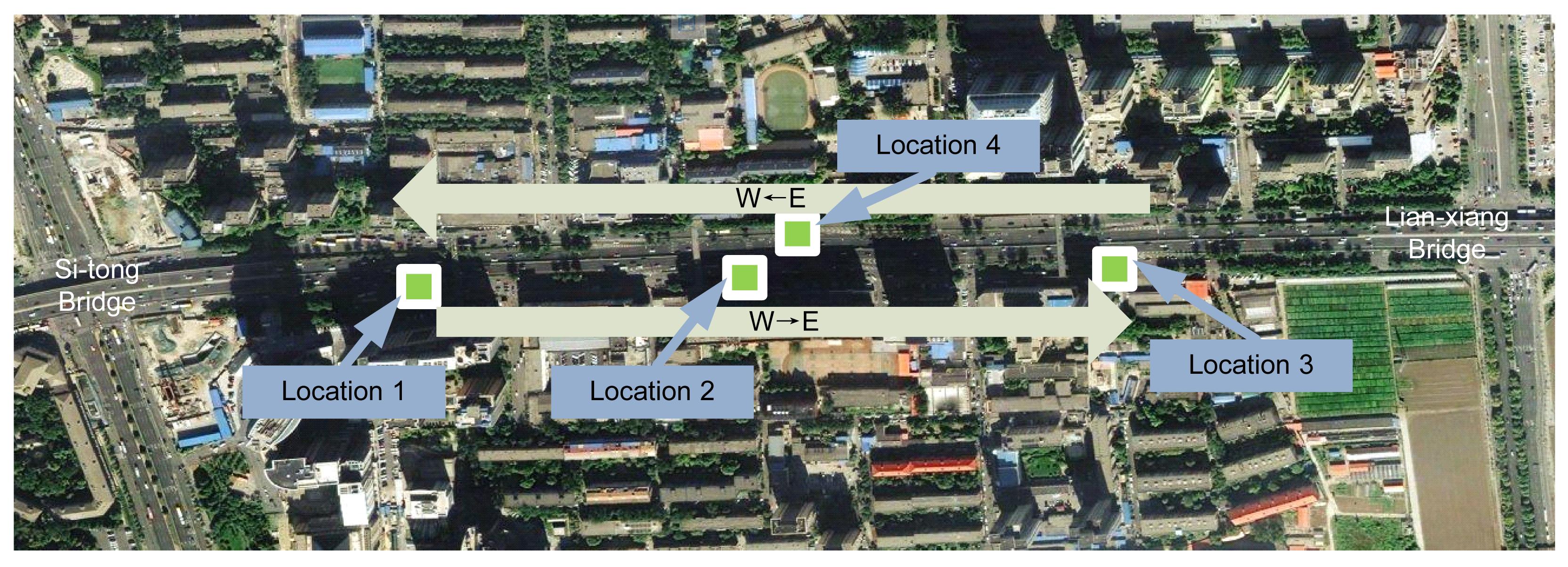
 The field TTC data analyzed in this study were collected by traffic management systems between Sitong Bridge and Lianxiang Bridge on the Beijing North Ring III expressway, China. The overhead Ring expressway is a vital infrastructure in Beijing’s road system, and has a total length of 48 km. The data were collected from four segment stations over a whole day, Tuesday, June 21, 2011. Station 1 is located on the mainline upstream of an on-ramp (direction W→E); station 2, in a weaving segment downstream of an on-ramp (direction W→E); station 3, on the mainline downstream of an off-ramp (direction W→E); and station 4, in a weaving segment downstream of an on-ramp (direction W←E) (Fig. 1). All segments of the selected expressway are three-lane roads, and the speed limit is 80 km/h. The datasets used to calculate the TTC values included every vehicle’s speed, time headway, and length.

2.3.  TTC characteristics

 To analyze the fundamental characteristics of the TTC samples, we used the raw traffic data from 6:00 am to 9:00 am (including morning peak hour and low volume periods) to calculate TTC values. Some fundamental statistical results for the four segments’ TTC values are shown in Table 1. The results show that 9101 TTC samples were collected with respect to the different road environments and traffic conditions. Each segment provided nearly 2275 TTC samples for the analysis. The TTC values in the different segments cover a very wide range, from 0.51 s to 69.82 s, and the standard deviations are large. The data clearly contain both low and high values of TTC, and even the very high values of TTC were included in the calculation of the means and variances. These statistics have more to do with traffic volume than traffic safety. For the purpose of traffic safety forecasting, we need to focus on the low TTC values that are significantly correlated with traffic conflicts.




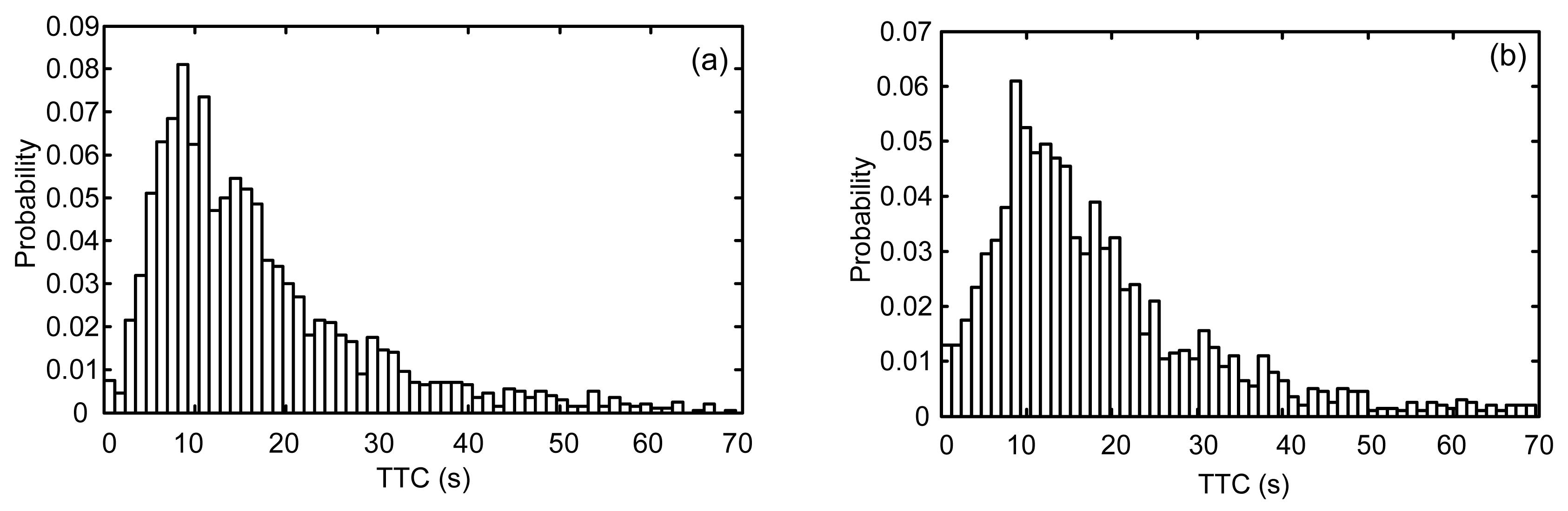
 To determine which TTCs should be included in our safety analysis, the proportion of short TTCs and the shape of the TTC distribution should be determined. Therefore, a common histogram method can be used first, with one predetermined bin-width. The simple histogram can provide brief but significant information about the TTC distribution. Fig. 2 illustrates the TTC distributions for two different segments. These examples indicate that the characteristics and variability of TTC distributions on different segments of a given expressway may have the same trends or patterns. Also, both samples seem to have multimodal and long-tailed distributions. This means that the TTC data may come from different unimodal distributions related to different levels of safety. One part of the data is concentrated around low TTC values (risky situations), while the other part is concentrated around high TTC values (safe situations). For the evaluation and prediction of traffic safety, we are more concerned about the TTC samples representing risky situations.

3.  GMM-based distribution of TTC

 In previous studies, TTC data have generally been described using a conventional probability density function (PDF), such as a normal, exponential, lognormal, gamma or inverse Gaussian distribution (Lord and Mannering, 2010). However, field TTC data from expressways have been shown to follow bimodal or multimodal distributions (Jin et al., 2011b). From the point of view of safety forecasting, TTC data representing risky and safe situations should follow different distributions, and there is no specific distribution function available to represent mixed TTC data covering both types of situation. Therefore, we need to use a more sophisticated method to model our TTC distribution.

 To estimate the PDFs (or parameters) of a mixed TTC distribution, the mixture model is a useful tool. The GMM, which is the most popular mixed distribution due to the simplicity of its estimation process, is a parametric PDF represented as a weighted sum of Gaussian component densities. The GMM can be represented by any type of probability distribution, and has been used widely for density estimation in computational, mathematical and optimization contexts. GMMs have been used successfully in a wide variety of fields, such as speaker recognition systems (Hsieh et al. 2003), video image processing (Stauffer and Grimson, 1999), pattern classification (Kim and Kang, 2007), and traffic safety parameter estimation (Jin et al., 2011b).

3.1.  Gaussian mixture model

 A GMM for the TTC distribution can be formed as follows, as a weighted sum of I component Gaussian distributions (Titterington et al., 1985): (3) , where P{TTC} represents the probability that a specific value, TTC, occurs, ω_i , i=1, 2, …, I, are the mixture weights, and , i=1, 2, …, I, with mean μ_i and variance σ_i ², are the component Gaussian density functions. Each component density is a univariate Gaussian function of the form: (4) . The mixture weights ω_i indicate the percentage of the TTC samples belonging to each category i and satisfy the constraint . The complete GMM is parameterized by the means, variances and mixture weights from all of the component Gaussian densities. These parameters are collectively represented by the notation .

 One of the powerful attributes of the GMM is its ability to form smooth approximations of arbitrarily shaped densities. Due to their ability to represent a large class of sample distributions, GMMs can be used to analyze TTC data and capture the component Gaussian distribution patterns. The use of a GMM to represent feature distributions of TTC data may also be motivated by the intuitive notion that the individual component densities may model some underlying set of hidden classes. For example, in the safety context, it is reasonable to assume that the TTC values correspond to different situations. The choice of model configuration (number of components and model parameters) is often determined by the amount of field data available for estimating the GMM parameters, and the specific application.

 In this study, TTC data could be classified into two categories (risky and safe) or three categories (such as high risk, medium risk and low risk), and a multimodal model could be developed accordingly based on similar methodology. The main contribution of this study is to propose this bi/multimodal concept to analyze TTC data. Therefore, for simplicity, two separate underlying regimes, leading to a mixture of two different Gaussian density distributions, were considered. The first mixture component, representing the low TTC values, depicts risky situations, while the second, representing the high TTC values, covers safe situations. Thus, in the case of this two-component GMM, the parameter I equals 2, the values of the mixture weights are associated with the safety of the traffic flow, and their sum should be 1.

3.2.  Maximum likelihood parameter estimation

 For the two-component GMM, five parameters need to be estimated. Given our TTC training samples, we wish to estimate the parameters of the GMM, θ, which in some sense best match the distribution of the training samples. There are several techniques available for estimating the parameters of a GMM (McLachlan, 1988). By far the most popular and well-established method is the maximum likelihood (ML) estimation. The aim of ML estimation is to find the model parameters that maximize the likelihood function of the GMM, given the training data. For a sequence of N TTC _j taken from the training data, the GMM likelihood function, assuming the independence of the TTC _j , can be written as (5) .

 The function is referred to as the likelihood of the parameters given the data, or simply the likelihood function. It is a function of the parameters θ for a fixed TTC. In the ML problem, the goal is to find the θ that maximizes L. That is, we wish to find θ ^* where, (6) .

 Unfortunately, this expression is a non-linear function of the parameters θ and direct maximization is not possible. However, a special case of the expectation-maximization (EM) algorithm can be obtained to estimate the ML parameters. The EM algorithm (Dempster et al., 1977) is a general method for finding the ML estimate of the parameters of an underlying distribution from a given dataset when the data is incomplete or has missing values. The basic idea of the EM algorithm is, beginning with initial parameters θ, to estimate new parameters , such that . The new parameters then become the initial parameters for the next iteration and the process is repeated until some convergence threshold or iteration number is reached.

 The EM algorithm first finds the expected value of the complete data log-likelihood. The evaluation of this expectation is called the E-step of the algorithm, and the second step (the M-step) maximizes the expectation computed in the first step. These two steps are repeated as necessary. Each iteration process is guaranteed to increase the log-likelihood, and the algorithm is guaranteed to converge to a local maximum of the likelihood function. For detailed descriptions of the EM algorithm, please refer to Redner and Walker (1984) and Jordan and Jacobs (1994).

3.3.  Results

 In this study, the GMM parameters are estimated from the TTC training data using the iterative EM algorithm, with the number of components I set to 2 in the empirical observation and analysis. The two categories of TTC data represent risky and safe situations, respectively. Two normal distributions are applied to fit the TTC data and the mixture weight of each distribution reflects the percentages of risky and safe situations in the traffic flow.

 Using the field samples from the four stations mentioned earlier, Table 2 shows the number of iterations of the EM algorithm, the estimated Gaussian distribution parameters, and the results of the Kolmogorov-Smirnov (K-S) test for each station. Looking at the values of the weights in each situation, we can see that the risky situations make up between 68% and 75% of the samples. The mean TTC values in risky situations are much lower than those in safe situations. Therefore, the GMM has the ability to distinguish between TTC samples in different situations and describe the characteristics of each Gaussian distribution.




 To verify further the fit of the results statistically, the K-S test was adopted as a goodness-of-fit test (Stephens, 1974). In statistics, the K-S test is a nonparametric test of the equality of continuous 1D probability distributions. It can be used to compare a sample with a reference probability distribution (one-sample K-S test), or to compare two samples (two-sample K-S test). The K-S statistic quantifies the distance between the empirical distribution function of the sample and the cumulative distribution function (CDF) of the reference distribution. The null distribution of this statistic is calculated under the null hypothesis that the sample is drawn from the reference distribution. As Table 2 shows, the K-S goodness-of-fit tests all suggested that the GMM performs well. The samples from the four stations are demonstrated to have been drawn from the GMM distribution at a statistical significance level of α=0.05.

 Fig. 3 depicts the EM estimation results for the two component Gaussian density function. It shows that the GMM has the ability to fit a two-peak distribution to the TTC data. The GMM fits the empirical data very well, with a small error. Fig. 3a shows the trends in the TTC based on the Gaussian mixture distributions using the TTC sample data from station 1. The mean TTC value is 10.51 s in the risky situations and 29.39 s in the safe situations, a difference of 18.88 s, and the mixing weights are 0.68 for risky situations and 0.32 for safe situations. The TTC pattern appears to follow a bimodal distribution since the mean difference between the two TTC regimes is large. Similarly, for station 2 (Fig. 3b), there is a large difference (17.59 s) between the means (9.82 s with a 0.73 mixing weight for the risky situations and 27.41 s with a 0.27 mixing weight for the safe situations), again indicating a two-peak distribution. Figs. 3c and 3d show similar patterns.

4.  Method of forecasting traffic safety

4.1.  Proportion of exposure to traffic conflicts

 In Section 3, the TTC distribution parameters representing risky situations, which are more significant for safety forecasting, have been extracted from the field data using GMM. However, we do not want to consider all of the TTC data relating to risky situations; instead, we should focus on the sample data that may lead to conflicts. Mainly for this reason, there is a need to develop the concept of the traffic safety indicator further and produce an assessment method that can be used indirectly to measure expressway traffic safety.

 For the purpose of safety forecasting, we define a new safety indicator: the proportion of exposure to traffic conflicts (PETTCs) in a given time period (e.g., 5, 10, or 15 min). PETTC represents the proportion of vehicles exposed to dangerous scenarios (or critical encounters). Having obtained the TTC distributions for the four expressway segments (Section 3), the PETTC in a particular interval can be defined as follows: (7) , where p _ettc is the PETTC, ω _rs is the weight, g _rs() is the CDF of that part of the TTC sample in risky situations, whose parameters can be estimated using the GMM and EM algorithm, and τ is a predetermined TTC threshold value.

 By introducing the probability concept in Eq. (7), the PETTC is easily obtainable once the TTC distributions are determined. Accordingly, PETTC (based on TTC) is a straightforward and useful indicator for forecasting traffic crashes in road sections. PETTC is thus the mixing weight for the risky situations multiplied by the probability that the TTCs in risky situations are lower than a predetermined threshold value. Therefore, the TTC threshold value is usually chosen to distinguish dangerous scenarios (or critical encounters) from relatively safe situations, and is of significance for the proposed new safety indicator. It is widely acknowledged that the TTC threshold should be between 2 and 4 s (Minderhoud and Bovy, 2001; Vogel, 2003). In this study, three conventional values (2, 3 and 4 s) are considered as possible TTC threshold values for safety forecasting.

 According to Meng and Qu (2012), there is a strong linear relationship between accident frequencies and conflicts. Therefore, PETTC is a good indicator for the potential risk of accidents and can be used for safety forecasting.

4.2.  Kalman filter

 Many different algorithms can be found in the literature that have being applied to time series forecasting (Khashei and Bijari, 2012), such as Bayesian networks (Park and Cho, 2012) and support vector regression (Jiang and He, 2012). These algorithms are complex and have little ability to predict online time-series data quickly. Therefore, in this paper, we propose a simple Kalman filter model for safety forecasting. The Kalman filter is an algorithm that operates recursively on streams of noisy input data to produce a statistically optimal estimate of the underlying system state. They have been applied in many areas, including navigation (Yim et al., 2011), water demand prediction (Nasseri et al., 2011), and traffic volume forecasting (Xie et al., 2007). An introduction to Kalman filter theory is given by Haykin (2001).

 The Kalman filter model assumes that the true state at step k evolves from the state at k−1 according to (8) , where represents the n-dimensional real variable domain, x _k and x _{k −1} are the state vectors at steps k and k−1, respectively, F _{k , k−1} is the state transition model which is applied to the previous state x_{k −1}, and w_k is the process noise, which is assumed to be drawn from a zero mean multivariate normal distribution with covariance Q _k , i.e., .

 At step k, a measurement (or observation) z _k of the true state x _k is made according to (9) , where represents the m-dimensional real variable domain. H _k is the measurement model that maps the true state space into the measured space, and v_k is the measurement noise, which is assumed to be zero mean Gaussian white noise with covariance R _k , .

 Let and represent the a priori and a posteriori state estimates at step k, respectively, of which the error covariance matrices are (10) , (11) .

 The Kalman filter process is shown in Fig. 4. The Kalman filter uses time update and measurement update algorithms to estimate x _k . First, a tentative estimate is calculated based on the value of ; then, the measurement value z _k is used to refine further the value of in order to obtain , which is the estimate of x _k .




 To forecast traffic safety using the Kalman filter, let p _ettc(k) denote the safety indicator, PETTC, for the kth time interval, that is to be estimated. It is assumed that the indicator p _ettc(k) at the time interval k has a linear relationship with the indicators at the last n intervals, as follows: (12) , where PETTC _k =[p _ettc(k−1), p _ettc(k−2), …, p _ettc(k−n)] is the measured safety indicator vector, is the collection of coefficients for each corresponding measured safety indicator in the row vector PETTC _k , and ε is the noise term.

 To implement the Kalman filter model, β _k is used as the state vector x _k in Eq. (8); PETTC _k is used as the measurement matrix H _k in Eq. (9); p _ettc(k) corresponds to z _k in Eq. (9); and Eq. (12) is equivalent to the measurement equation shown in Eq. (9). Assume now that there are n+1 observed safety indicators: p _ettc(k), p _ettc(k−1), …, p _ettc(k−n). Based on the Kalman filter prediction algorithm illustrated in Fig. 3, first the a priori estimate of β _k is calculated ( ), then the measured value of p _ettc(k) is used to update and obtain an a posteriori estimate Since, for short-term forecasting, the transition of the state vector can be regarded as a smooth process, the safety indicator at the next time interval can then be predicted by (13) .

 Several parameters need to be determined before starting the recursive Kalman filter prediction process. The transition matrix F _{k ,k−1} is set to be an n×n identity matrix since the transition is generally smooth. The calculated PETTCs can be used as the true safety indicator values so it is assumed that there is no measurement error and the variance of the measurement noise, R , is zero. The variance of the process error, Q , is obtained by minimizing the following negative log-likelihood function (Digalakis et al., 1993). (14) , where , C is the constant value and M is the number of sample intervals.

 Based on the algorithm outlined in Fig. 4, the traffic safety prediction for the expressway using the Kalman filter is carried out as follows:

1. Let k=n+1 set initial values for . P _{k −1} is customarily set to be a matrix with very small values. In this study, is set to be [1/n, 1/n, …, 1/n]^T and P _{k −1}=10⁻² I _n×n .

2. Calculate and using the equations shown in the time update (predict) part of Fig. 4.

3. Let H _k =[p _ettc(k−1), p _ettc(k−2), …, p _ettc(k−n)] and z_k =p _ettc(k). Calculate K , and P _k using the equations shown in the measurement update (correct) part of Fig. 4.

4. Let H _{k +1}=[p _ettc(k), p _ettc(k−2), …, p _ettc(k−(n−1))], then the predicted value of .

5. Let k=k+1 and go to step 2.

4.3.  Forecasting process and performance evaluation

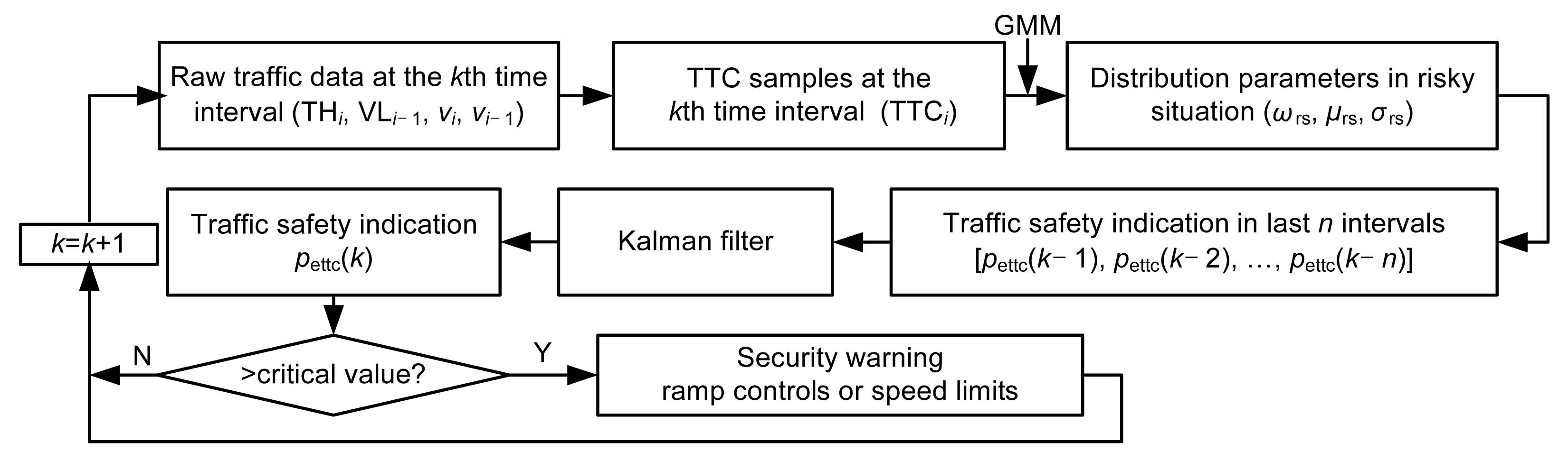
 The main idea in this study is to apply a Kalman filter model to estimate the safety indicator PETTC. Fig. 5 shows a flowchart of the traffic safety forecasting procedure. The process includes five main steps: (1) raw traffic data are used to calculate TTC values in each time interval, (2) TTC distribution parameters are obtained based on the GMM, (3) a new traffic safety indicator (PETTC) is calculated using the TTC distribution parameters, (4) a Kalman filter model is applied to predict the PETTC values in the next interval, and (5) it is determined whether the PETTC is larger than a predetermined threshold; if so, a security warning is reported and management and control technologies, such as ramp controls or speed limits, are applied to lower the traffic risk.




 As discussed above, this study aims to forecast a safety indicator at short intervals, and a 30-min interval was chosen. Since volumes of traffic early in the morning and late at night are very small, the number of TTC data points is also small, and this period is typically of little concern to researchers. Therefore, only data from 5:00 am to 11:00 pm (a total of 18 h and including 36 time intervals) were used for prediction and performance evaluation.

 We employed two commonly used performance indices to evaluate the proposed online forecasting model. The first was the mean absolute percentage error (MAPE), and the second was the root mean square error (RMSE). These indices are given by the following equations: (15) , (16) , where M is the number of sample intervals.

4.4.  Results and analysis

 Based on the above flowchart, we calculated the predicted safety indicators for the four stations. Fig. 6 shows scatter plots of the measured and predicted PETTC values, from which it can be seen that the predicted data fit the measured data well, both in low-risk and high-risk situations. The gap between the measured and predicted results throughout the whole domain is small. Therefore, the proposed model, based on the GMM and the Kalman filter, can be seen to be a very accurate and robust online prediction method for short-term traffic safety forecasting.




 Table 3 shows the performance indices of the proposed prediction model. These results indicate that the average MAPE value is about 5.0% and the average RMSE value about 0.00136, and that our prediction method can accurately forecast traffic safety indicators for all four datasets and different TTC threshold values. It is easy to see that the MAPE and RMSE values are both stable and robust, which supports the theory that it is effective to use the safety indicator, PETTC, to improve short-term traffic safety predictions. Therefore, this method can be applied for the online forecasting of relative changes in levels of safety for different road environments or traffic conditions.

5.  Summary

 Traffic safety prediction is of great significance for the optimal operation of expressway traffic management systems. Accurate and timely online traffic safety prediction can help managers to identify traffic risks quickly, and reduce these risks using ramp controls or speed limits. Therefore, forecasting traffic safety is one of the most important functions of expressway traffic management systems. In this paper, we propose a GMM and Kalman filter-based online traffic safety forecasting method. Firstly, the raw traffic data are used to calculate TTC values at 30-min intervals, and the statistical characteristics of the TTC sample values are presented. Secondly, the Gaussian mixture distribution is used to fit the empirical distributions of the TTC samples, which seem to be bimodal. Therefore, we can use the two-component GMM, and apply the EM algorithm to estimate the TTC distribution parameters. Then, a new traffic safety indicator, the PETTC, is proposed for risk assessment and safety predictions for expressway traffic. This indicator is demonstrated to have a strong correlation with accident frequencies, and can easily be obtained from traffic management systems. A Kalman filter-based prediction model is proposed for online short-term safety forecasting, and a detailed flowchart of the process is presented. Finally, datasets collected from four different locations on the Beijing expressway are used for performance estimation. The results show that the MAPE value is about 5.0% and the RMSE value about 0.00136. The test results demonstrate that the proposed algorithm performs well in online safety forecasting. Further studies could use a more complex prediction model, such as the extended Kalman filter, neural networks, or the discrete wavelet, to improve the performance further.

---

* Project (No. 2011AA110304) supported by the National High-Tech R&D Program of China (863 program)