Affiliation(s):
. Key Laboratory of Advanced Control and Optimization for Chemical Processes of Ministry of Education, East China University of Science and Technology, Shanghai 200237, China
Chu-dong Tong, Xue-feng Yan, Yu-xin Ma. Statistical process monitoring based on improved principal component analysis and its application to chemical processes[J]. Journal of Zhejiang University Science A, 2013, 14(7): 520-534.
@article{title="Statistical process monitoring based on improved principal component analysis and its application to chemical processes", author="Chu-dong Tong, Xue-feng Yan, Yu-xin Ma", journal="Journal of Zhejiang University Science A", volume="14", number="7", pages="520-534", year="2013", publisher="Zhejiang University Press & Springer", doi="10.1631/jzus.A1300003" }
%0 Journal Article %T Statistical process monitoring based on improved principal component analysis and its application to chemical processes %A Chu-dong Tong %A Xue-feng Yan %A Yu-xin Ma %J Journal of Zhejiang University SCIENCE A %V 14 %N 7 %P 520-534 %@ 1673-565X %D 2013 %I Zhejiang University Press & Springer %DOI 10.1631/jzus.A1300003
TY - JOUR T1 - Statistical process monitoring based on improved principal component analysis and its application to chemical processes A1 - Chu-dong Tong A1 - Xue-feng Yan A1 - Yu-xin Ma J0 - Journal of Zhejiang University Science A VL - 14 IS - 7 SP - 520 EP - 534 %@ 1673-565X Y1 - 2013 PB - Zhejiang University Press & Springer ER - DOI - 10.1631/jzus.A1300003
Abstract: In this paper, a novel criterion is proposed to determine the retained principal components (PCs) that capture the dominant variability of online monitored data. The variations of PCs were calculated according to their mean and covariance changes between the modeling sample and the online monitored data. The retained PCs containing dominant variations were selected and defined as correlative PCs (CPCs). The new Hotelling’s T2 statistic based on CPCs was then employed to monitor the process. Case studies on the simulated continuous stirred tank reactor and the well-known tennessee Eastman process demonstrated the feasibility and effectiveness of the CPCs-based fault detection methods.
Darkslateblue:Affiliate; Royal Blue:Author; Turquoise:Article
Article Content
1. Introduction
Multivariate statistical methods, such as principal component analysis (PCA) and partial least squares (PLS), are widely used in industry for process monitoring (Nomikos and MacGregor, 1995; Qin, 2003; Ge and Song, 2008; Garcia-Alvarez et al., 2012). Other complementary multivariate statistical process monitoring methods, including canonical variate analysis, kernel PCA, dynamic PCA, and independent component analysis, have been proposed to address the limitations of PCA- or PLS-based monitoring strategies (Russell et al., 2000; Juricek et al., 2004; Lee et al., 2004a; 2006). PCA-based and related monitoring methods, which build statistical models from normal operation data and partition the measurements into a principal component subspace (PCS) and a residual subspace (RS), are among the most widely used multivariate statistical methods. In this methodology, the dimension of the PCA model, which is the estimation of the optimal number of principal components (PCs) to retain, must be determined and has an important role on the process monitoring performance. However, the determination of the number of PCs is not unique, given that the sensor outputs are generally disturbed by noise (Tamura and Tsujita, 2007).
The choice of PCs is a crucial step for the interpretation of monitoring results or subsequent analysis because it could lead to the loss of important information or the inclusion of undesirable interference. To tackle this challenge, a large number of well-known techniques for selecting the number of PCs have been proposed. A simple approach is to choose the number of PCs for the variance to achieve a predetermined percentage, such as 85%, termed as cumulative percent variance (CPV) (Jackson, 1991). Other methods for determination, including cross validation, average eigenvalue approach, variance of reconstruction error (VRE) criterion, and fault signal-to-noise ratio (fault SNR), have been proposed to determine the number of the retained PCs (Wold, 1978; Dunia and Qin, 1998; Valle et al., 1999; Tamura and Tsujita, 2007). The cross validation method uses part of the training samples for the model construction, while the rest are compared with the prediction by the model. However, this criterion needs to build multi-PCA models, which is tedious. The average eigenvalue approach accepts all the eigenvalues with values of above the average eigenvalue and rejects those below the average. This criterion is simple, but comparatively robust. The VRE criterion assumes that the corresponding PCs are deemed as the optimal PCs when the error of fault reconstruction comes to minimum. Fault SNR shows the relationship between the number of PCs and the fault detection sensitivity, which maximizes the sensitivity of fault detection. When a priori knowledge of the fault direction is available, both methods can determine the optimal number of PCs for the fault detection from different perspectives.
Several comparative studies have been conducted on these methods for determining the number of PCs for the fault detection. Valle et al. (1999) tested 11 methods and concluded that the VRE criterion is preferable. Tamura and Tsujita (2007) compared fault SNR with VRE criterion, and concluded that these two methods calculate different characteristics depending on the analysis objective. In addition, both methods need a fault direction vector as a priori process knowledge, which is hardly obtained in practical applications, especially for complex chemical processes. Nevertheless, the determination of the retained PCs of these traditional approaches is rather subjective or requires a priori knowledge, and none of these methods considers the performance of the fault detection in the absence of a priori knowledge. Apart from these comparative studies, the fault detection ability depends on the PCs retained in the PCA model (Kano et al., 2002). Togkalidou et al. (2001) indicated that including components with smaller eigenvalues in the PCA model and excluding those with larger eigenvalues can improve the prediction quality. Motivated by this perspective, the present work deals with several of the limitations inherently associated with most of the traditional criterions for determining the retained PCs.
When the PCA model is employed for monitoring industrial processes, Hotelling’s T2 and squared prediction error (squared prediction error (SPE) or Q) statistics are usually used for the fault detection. T2 index is the squared Mahalanobis distance of the projections in PCS, designed to measure the variability of the mean and covariance within the PCS. Given each PC is the linear combination of original data, the variability of the original data may be submerged in several projection directions with larger variance considering small coefficients corresponding to the measured variables. In the following section, the monitoring components with relatively small eigenvalues have been shown to result in a better fault detection performance. Similar to the statement presented by Togkalidou et al. (2001), the basis of the proposed method is that the first l PCs that capture the dominant variance of the modeling data may not best reflect the variability of the online monitored data samples, and thus a number of special faults cannot be well detected.
In this work, a novel criterion is introduced to determine the retained PCs objectively and dynamically. This method differs from the traditional approaches mentioned above, in which the selected PCs can capture the dominant variability (mainly the changing of mean and covariance) of the online observations against the modeling data, instead of capturing cumulative variance. The online measurements lead to variation within PCS, and the degree of variability captured by each component can be evaluated according to a predefined criterion through a moving-window technique. The PCs that contain the dominant variability is selected for the fault detection, which is termed as correlative PCs (CPCs) in this paper. With the embedding of the moving window, no prior knowledge of the abnormal situations is needed, and the selected components can expose the variability of the current samples to maximum. The contributions of the proposed method are as follows.
Unlike the traditional criterion, the proposed approach determines the retained PCs objectively, without the restriction that the components corresponding to larger eigenvalues should be selected. CPCs are similar to PCs containing the dominant variance of the modeling data when the current samples are normal. For potential abnormal observations, the CPCs can be automatically determined to be those that capture the main variability. Therefore, the PCA model parameter that accounts for the fault detection can be chosen, and the monitoring performance can subsequently be improved.
Although fault SNR and VRE criterion can determine the number of PCs objectively, a prior knowledge of the fault direction is required, which may induce redundant information for the fault detection inevitably. In the proposed method, prior knowledge is not necessary and CPCs can be determined dynamically according to the variations caused by the current window.
Compared with the conventional PCA-based method, SPE statistic is eliminated in the improved PCA-based approach considering that the variability of online observations is mainly contained in CPCs and the one-fold T2 index is enough for monitoring the industrial processes. Moreover, a single index can provide the operators more precise information without any confusion.
2. PCA-based process monitoring
2.1. Preliminaries of PCA
One of the most popular methods for dealing with multivariate data is PCA, which transforms a correlated original data to uncorrelated data set, while preserving the most important information of the original data set (Jackson, 1991). PCA includes the decomposition of data matrix X∈ which contains n regular-sampled observations of m process variables and is scaled to zero mean and unit variance, into a transformed subspace of reduced dimension. The decomposition is expressed as follows: , where X∈ and P∈ are the score matrix and the loading matrix, respectively. The matrices and E
represent the estimation of X and the residual part of the PCA model, respectively, which are defined as follows: , .
The principal component projection reduces the original set of variables to l PCs. The decomposition assumes that is orthonormal and is orthogonal. The columns of P are actually the eigenvectors of the covariance or correlation matrix, R, associated with m eigenvalues [λ1, λ2, …, λm] (the eigenvalues are listed in descending order). Alternatively, the matrix X can be decomposed using singular value decomposition to build the PCA model. The number of PCs, l, is a key parameter in the PCA model and is commonly determined using the CPV method, cross validation, and average eigenvalue approach, as mentioned above.
The procedures of the conventional PCA to perform process monitoring are introduced in this subsection. A new sample vector x (after scaling with the mean and variance obtained from the normal data) becomes available and is projected with the help of the PCA model to either PCS or RS. Two statistics, namely, Hotelling’s T2 and SPE (or Q), have been developed for process monitoring (Chiang et al., 2001). T2 is the Mahalanobis distance of a score vector, t, in the PCS, and Q is the Euclidean distance of a residual vector in the RS, which are given by , , where Λ=diag{λ1, λ2, …, λl}, e is the residual vector, and I∈ denotes identity matrix. Therefore, the scalar thresholds can qualify the process status. The approximated control limits of T2 and Q statistics, with a confidence level α, can be determined from the normal operating data in several ways by applying the probability distribution assumptions (Kourti and MacGregor, 1995; Qin, 2003). The control limits can be calculated as follows: , , where Fα(l, n−l) is the upper limit of α percentile of the F-distribution with the degree of freedoms l and n−1, cα is the normal distribution value with the level of significance α, and , .
In general, T2 statistic measures the significant variability within the PCs, while Q indicates how well the reduced dimensional PCA model can describe the significant process variation. In most cases, Q is considered as an assistant statistic for T2 considering that the value of Q can be significantly affected by the process noise. The process condition is considered abnormal if the statistics of a new observation exceed the control limit.
2.2. Motivation analysis
In this subsection, a simple multivariate process (Lee et al., 2004b), which is a modified version of the system suggested by Ku et al. (1995), is considered to illustrate the motivation analyses: , , where u is a correlated input expressed as .
The input w is a random vector, in which each element is uniformly distributed on the interval (−2, 2). The output y is equal to z plus a random noise, v. Each element of v has zero mean and 0.1 variance. Both input u and output y are measured, but not z and w. The basic data vector for the monitoring at step k consists of x(k)=[u1, u2, y1, y2, y3]T. The following abnormal case is considered to reveal the defect of the traditional criterions.
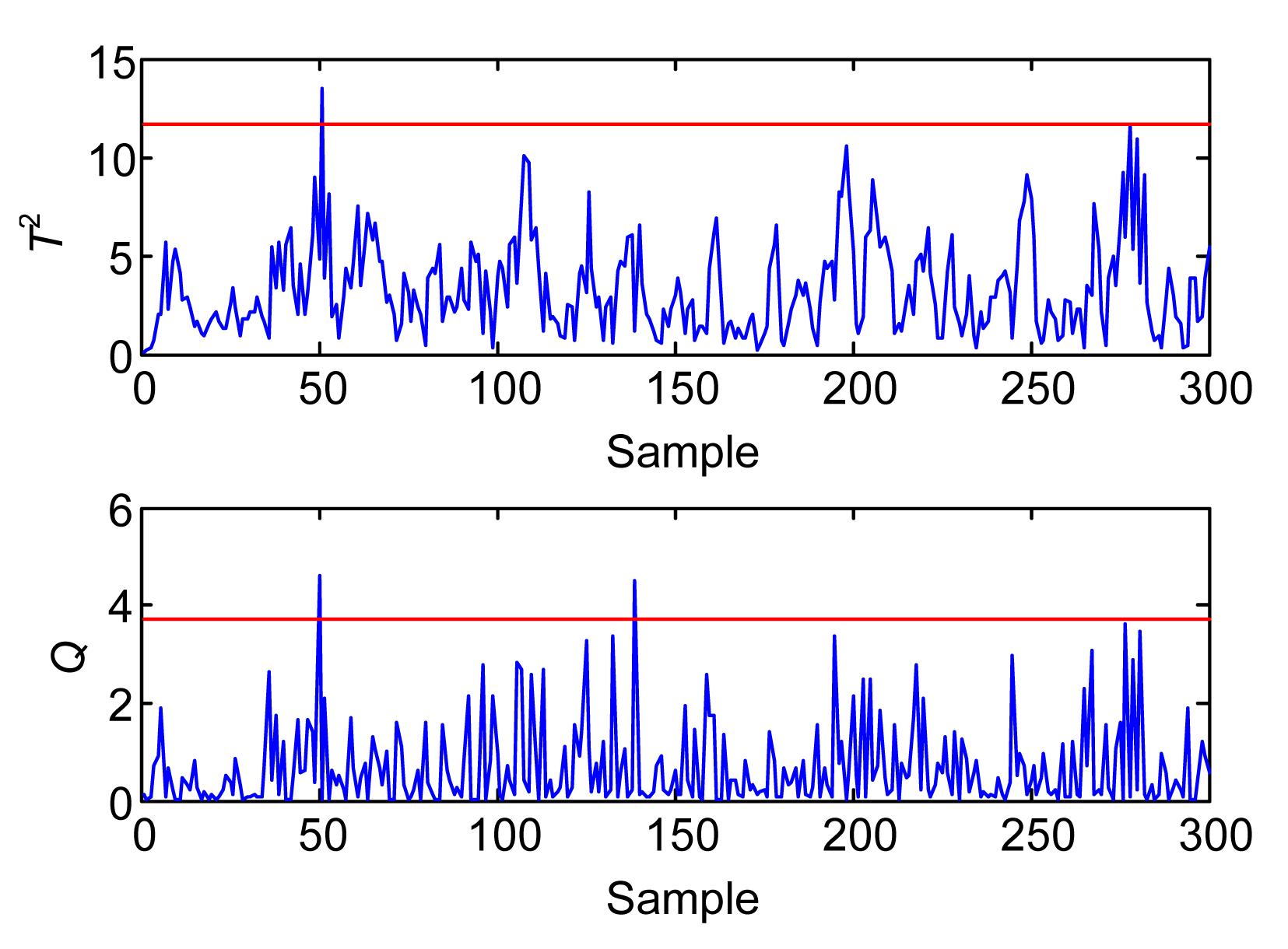
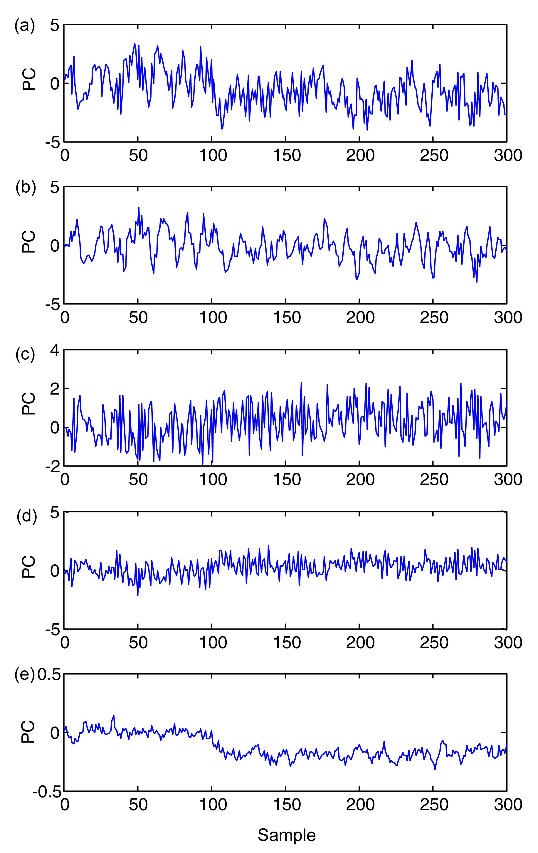
In PCA, a three-principal component model has been developed on 300 normal samples, which captured about 87% of the process variance. For testing purpose, a step change of 2 is introduced to w1 starting from sample 100 to the end of operating duration. The T2 and Q charts of the process with this disturbance are shown in Fig. 1, as well as the 99% confidence limits. However, PCA cannot detect the disturbance and captures only the dominant randomness. By contrast, the occurrence of abnormality is mainly captured by the first and the fifth PCs based on the plots of the five PCs of the online samples given in Fig. 2. With the inclusion of unnecessary information and the elimination of several components corresponding to relatively small eigenvalues, the T2 and Q derived from the first three PCs did not show considerable departure from the normal status. Therefore, fault detection must be considered in determining the retained PCs.
Fig.1 Monitoring result based on conventional PCA
Fig.2 Time-series plots of 1st PC (a), 2nd PC (b), 3rd PC (c), 4th PC (d), and 5th PC (e)
3. CPCs for the fault detection
Chemical process is often characterized by large scale and process data projected onto the loading matrix often marked with irrelevant information for the fault detection. Although the T2 statistic of the first l PCs can show deviation from the normal values in PCS, it still suffers from irrelevant PCs and low computational efficiency. Thus, selecting several PCs that indicate significant variation of the online observations in reduced subspace can improve the monitoring performance of the conventional PCA method. The selected PC is defined as CPCs, as mentioned above. The definition of CPCs is presented in the following subsection.
3.1. Definition of CPCs
For Hotelling’s T2, the variations of the mean and the covariance matrix are generally two essential factors that represent the process changes from a normal situation to a situation with several faults (Kresta et al., 1991). Each PC’s contribution to the T2 index comes from two parts, namely, the mean or variance change of the PC itself and the relationship with other PCs responsible for the process change. Recently, cumulative percent variation (He et al., 2009) based on each variable’s equivalent variation has been proposed to determine the candidate variables as follows: , where xj(i) is the ith element of the jth observation, b0(i) is the ith element of the normal mean vector b0, δ0(i) is the standard deviation of the ith variables of the normal data set X0, and ri is the ith column of the correlation matrix of the fault data set X. The index shows that each variable’s maximum variation comes from the mean or variance change of either the variable itself or the other variables related with the variable.
In this work, a similar index is defined to calculate the maximum variation of ith PC for online samples. In addition, a moving window is adopted to update the current data matrix, that is, the newest sample was augmented to the data matrix, whereas the oldest sample is discarded to keep a fixed number of samples in the data matrix. Let the kth data matrix with window length d be X=[xk−d+1, xk−d+2, …, xk]T∈, and then Tk=[tk−d+1, tk−d+2, …, tk]T∈ is obtained by projecting Xk onto the loading matrix P. For normal modeling data set X0, the corresponding score matrix T0=[t1, t2, …, td]T is used as reference matrix. The following index has been adopted to calculate each PC’s contribution to the process change: , where tj(i) is the ith element of the jth score vector in Tk, and is the standard deviation of the ith PCs of X0, which is equal to the ith eigenvalue. ri is the ith column of the correlation matrix, R, of Tk. S0 and Sk are the covariance matrices of T0 and Tk, respectively, which are given by , . Sk utilizes the mean vector b0 of the reference score matrix T0, which is a zero vector, and indicates the change in the covariance matrix more clearly. (Sk−S0)i is the ith column of (Sk−S0). Eq. (14) has two parts. The first part shows the mean change and the mean change induced by other variables. The other part represents the equivalent covariance change. After calculating all the PCs’ maximum variations, they are ranked in a decreasing order. The first several PCs sufficient to express the dominant change information of the current data matrix from the normal data set are determined as CPCs. In this step, the CPCs can be obtained by calculating the cumulative percent variation as follows: . Cumulative percent variation is a measurement of the percent variation captured by the first l ordered PCs, similar to CPV. We use D to denote the cumulative percent variation to avoid the confusion of this index with CPV. These two indices calculate different characteristics depending on the analysis objective. The first l PCs are defined as CPCs. The number of CPCs can be determined when D reaches a predetermined limit η, and we suggest that 65%≤η ≤70%. Moreover, when the data set Xk contains no abnormal sample data and the PCs have insignificant mean or variance change, they share similar variation along all PCs.
3.2. Process monitoring procedures
Given that the CPCs are determined by computing the correlation and covariance matrices of the score matrix of the current data set Xk, their adaptation suffer from low computational efficiency. Wang et al. (2005) proposed a fast-moving-window algorithm for adaptive process monitoring, which incorporates the adaptation technique in a recursive PCA algorithm (Li et al., 2000) and performs through a two-step procedure to calculate the correlative matrix efficiently. In this study, the same idea is introduced to update the correlation and covariance matrices of the current score matrix to increase computational efficiency. The full details of the calculation are described in the Appendix.
A real-time monitoring scheme can be implemented efficiently using the presented two-step algorithms. First, a sufficient large number of normal observations are necessary to obtain the PCA model. When the initial size of online observations reaches the prescribed window length, they are projected onto the loading matrix P to obtain the score matrix. ΔT(i) is then calculated for each PC, and the CPCs for the process monitoring are determined using the index D. Subsequently, the time-window is moved to the next step when a new sample is measured. The fast algorithm is applied to update the covariance and correlative matrices efficiently, and the CPCs for the next data matrix are determined. The consistent threshold for monitoring statistics is prescribed according to the number of CPCs for each time-window. The monitoring statistic used is Hotelling’s T2 statistic. Given that all the PCs of the significant variation are incorporated into T2 and the remainders have little deviation from the normal data, calculating the SPE statistic is unnecessary.
The complete monitoring procedures of the improved PCA with CPCs are summarized as follows.
Off-line modeling:
(1) Sufficient data are acquired when a process is operated under a normal condition. Each column (variables) of the data matrix is normalized, i.e., scaled to zero mean and unit variance.
(2) PCA is applied to the data matrix, and the loading matrix P∈ and the eigenvalue matrix D=diag{λ1, λ2, …, λm} are obtained.
(3) The size of time-window, d, and the threshold of cumulative percent variation, η are determined.
Online monitoring:
When the online observations become available, the monitoring task is initiated after the number of the new process data reaches d. The CPCs for the first time-window are used for monitoring all of the d observations, whereas the CPCs for the subsequent data matrix are only used for monitoring the new added data point.
(1) For online monitoring, the data matrix Xk representing the current operating conditions is updated by moving the time-window step by step and is scaled based on the mean and the variance obtained at Step 1. Subsequently, they are projected onto P to obtain the score matrix Tk, and ΔT(i) is computed for each PC using Eq. (14).
(2) The values in the vector ΔT are ranked, and the first l PCs that capture the dominant variability of the current score matrix Tk are set as the CPCs according to Eq. (17). The Hotelling’s T2 statistic of the CPCs is computed. The control limit is then calculated according to the number of CPCs dynamically.
(3) If the T2 statistic is under the control limit, the process is judged as normal and the time-window is moved to the next step. Conversely, if the T2 statistic is outside the control limit, the new added data point is considered as abnormal, and the fault diagnosis method is used to analyze the fault roots.
4. Case study
4.1. Continuous stirred tank reactor (CSTR) simulation
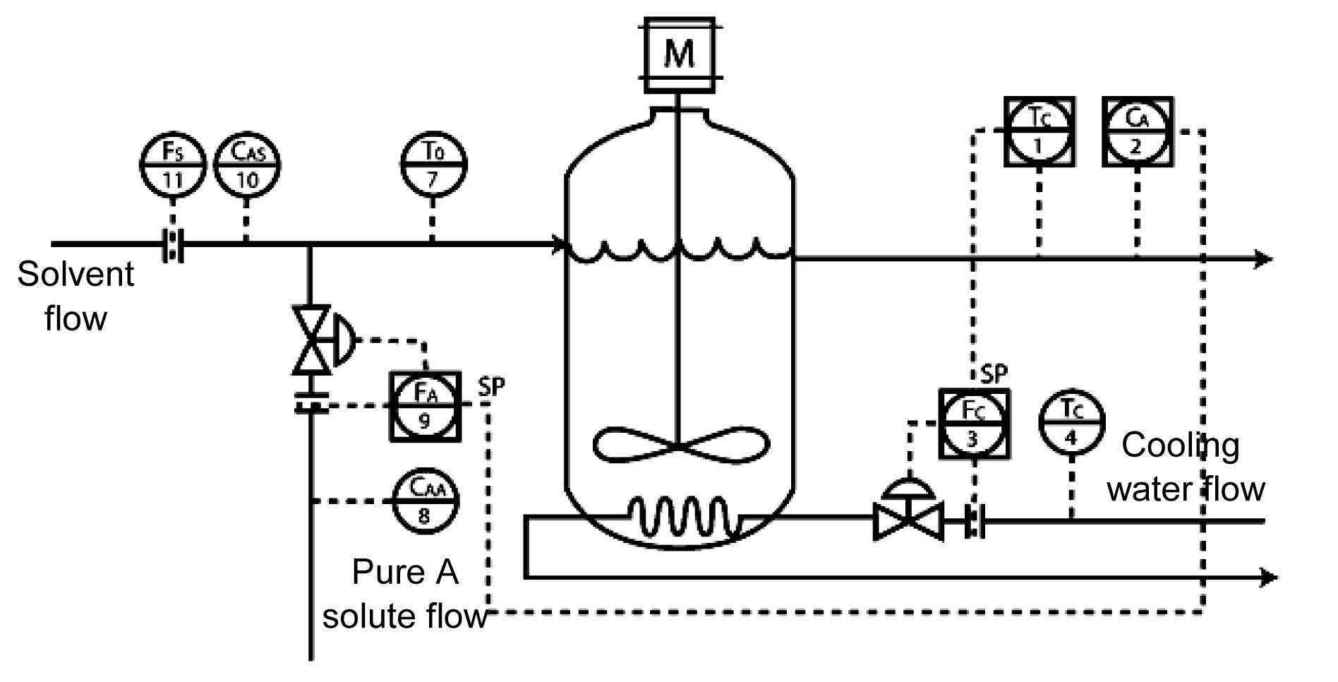
In this section, a continuous stirred tank reactor (CSTR) is simulated. The process model is similar to that provided by Yoon and MacGregor (2001). A diagram of the process is shown in Fig. 3. The simulation is performed according to the following model: , , where k0, E, and ΔHrxn are the pre-exponential constant, activation energy, and enthalpy of the reaction, R is the gas constant, cp and ρ are the heat capacity and density of the fluid in the reactor. The process is monitored to measure the cooling water temperature TC, inlet temperature T0, inlet concentrations CAA and CAS, solvent flows FS, cooling water flow FC, outlet concentration CA, temperature T, and reactant flow FA. The detailed model information and simulation parameters are provided in (Alcala and Qin, 2010). The measurements are sampled every minute, and the 1000 samples taken under normal conditions are used as the training data set. For fault cases, the test data sets also comprise 1000 samples, with the fault introduced after the 200th sample.
Fig.3 Diagram of the CSTR process
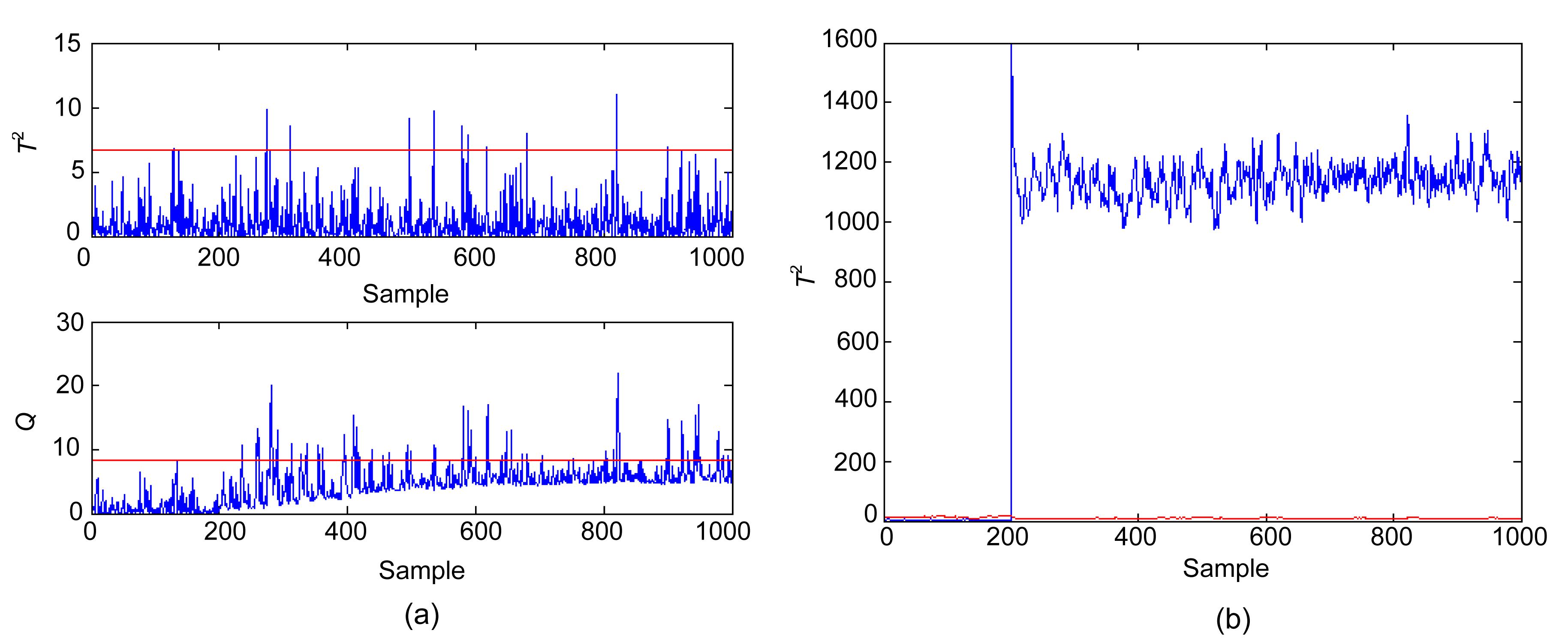
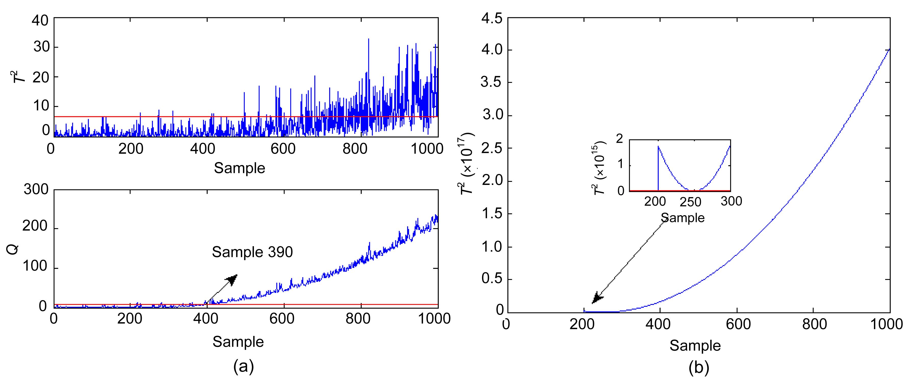
Two different faults are studied in this work. The first simulated fault, Fault 1, is a bias in the sensor of the output temperature T, with a bias magnitude of 0.05. Given that T is a controlled variable, the effect of the fault will be removed by the proportional-integral controller, and its effect will propagate to other variables. This fault is considered as a complex fault because it affects several variables. The monitoring results of the conventional PCA-based method and the proposed method are illustrated in Figs. 4a and 4b, respectively. The retained number of PCs for PCA is determined using the CPV criterion, with the cutoff value of 85%. The superiority of the proposed method for fault detection can be easily observed. Fault 2 is a drift in the sensor of CAA and its magnitude is kmol/(m3·min); thus, this is a simple fault. The conventional PCA-based method detects this fault with a delay of 190 min, as shown in Fig. 5. The improved PCA-based method can successfully and consistently detect the fault.
Fig.4 Monitoring results of Fault 1 of the conventional PCA (a) and improved PCA (b)
Fig.5 Monitoring results of Fault 2 of the conventional PCA (a) and improved PCA (b)
4.2. Tennessee Eastman (TE) process
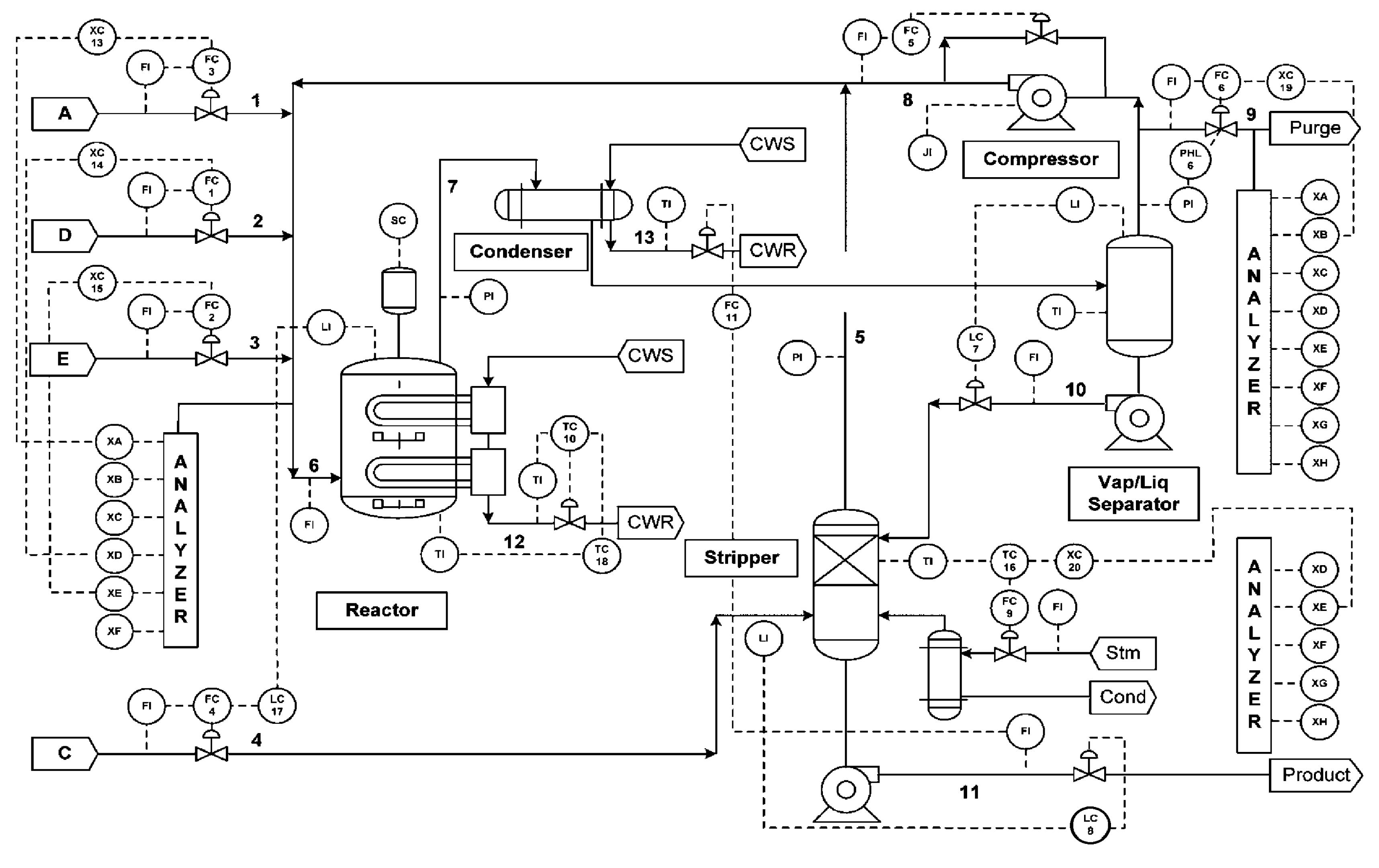
TE process is a well-known benchmark for testing the performance of various fault detection methods (Lyman and Georgakist, 1995; Yu and Qin, 2008; Liu et al., 2010; Chen and Yan, 2012; Stubbs et al., 2012). A flowchart of the TE process is shown schematically in Fig. 6. There are five major unit operations in the process: a reactor, a condenser, a recycle compressor, a separator, and a stripper. Four reactants A, C, D, E, and inert B are fed to the reactor where the products G and H are formed and a by-product F is also produced. The process has 22 continuous process measurements, 12 manipulated variables, and 19 composition measurements sampled less frequently. Details on the process description are well explained in (Chiang et al., 2001). A total of 33 variables are used for monitoring in this study as shown in Table 1. All composition measurements are excluded since they are hard to measure online in practice.
Fig.6 Tennessee Eastman process benchmark
Table 1
Monitoring variables in the TE process
No.
Process measurement
1
A feed
2
D feed
3
E feed
4
Total feed
5
Recycle flow
6
Reactor feed rate
7
Reactor pressure
8
Reactor level
9
Reactor temperature
10
Purge rate
11
Product separator temperature
12
Product separator level
13
Product separator pressure
14
Product separator underflow
15
Stripper level
16
Stripper pressure
17
Stripper underflow
18
Stripper temperature
19
Stripper steam flow
20
Compressor work
21
Reactor cooling water outlet temperature
22
Separator cooling water outlet temperature
23
D feed flow valve
24
E feed flow valve
25
A feed flow valve
26
Total feed flow valve
27
Compressor recycle valve
28
Purge valve
29
Separator pot liquid flow valve
30
Stripper liquid product flow valve
31
Stripper steam valve
32
Reactor cooling water flow
33
Condenser cooling water flow
The detailed description of the programmed faults (Faults 1–21) is listed in Table 2. The data are generated at a sampling interval of 3 min and can be downloaded from http://brahms.scs.uiuc.edu. For comparison, 960 normal samples are used to build the model. Another 500 normal samples are used for the validation. Each fault data set contains 960 samples, with the fault introduced after sample 160.
Table 2
Process faults for the TE process
Fault
Description
Type
1
A/C feed ratio, B composition constant (stream 4)
Step
2
B composition, A/C ratio constant (stream 4)
Step
3
D feed temperature (stream 2)
Step
4
Reactor cooling water inlet temperature
Step
5
Condenser cooling water inlet temperature
Step
6
A feed loss (stream 1)
Step
7
C header pressure loss-reduced availability (stream 4)
Step
8
A, B, C feed compositions (stream 4)
Random variation
9
D feed temperature (stream 2)
Random variation
10
C feed temperature (stream 4)
Random variation
11
Reactor cooling water inlet temperature
Random variation
12
Condenser cooling water inlet temperature
Random variation
13
Reaction kinetics
Slow drift
14
Reactor cooling water valve
Sticking
15
Condenser cooling water valve
Sticking
16
Unknown
Unknown
17
Unknown
Unknown
18
Unknown
Unknown
19
Unknown
Unknown
20
Unknown
Unknown
21
The valve for stream 4 was fixed at the steady-state position
Constant position
The proposed method is applied to the TE process simulation data and its fault detection performance is compared with conventional PCA monitoring strategy that utilizes the subjective method (i.e., CPV, cross-validation) to select PCs. A total of 18 faults have been tested in the TE process. Faults 3, 9, and 15 have been suggested to be difficult to detect (Russell et al., 2000; Lee et al., 2006; Wang and He, 2010), which is also confirmed in this study.
Therefore, they are not considered in this study. The normal training data set has 960 observations, which is used for PCA modeling. The loading matrix P∈ is obtained. The dimension of the reduced subspace is determined using the CPV method, in which the CPV value is larger than 85% when the number of PCs is 14.
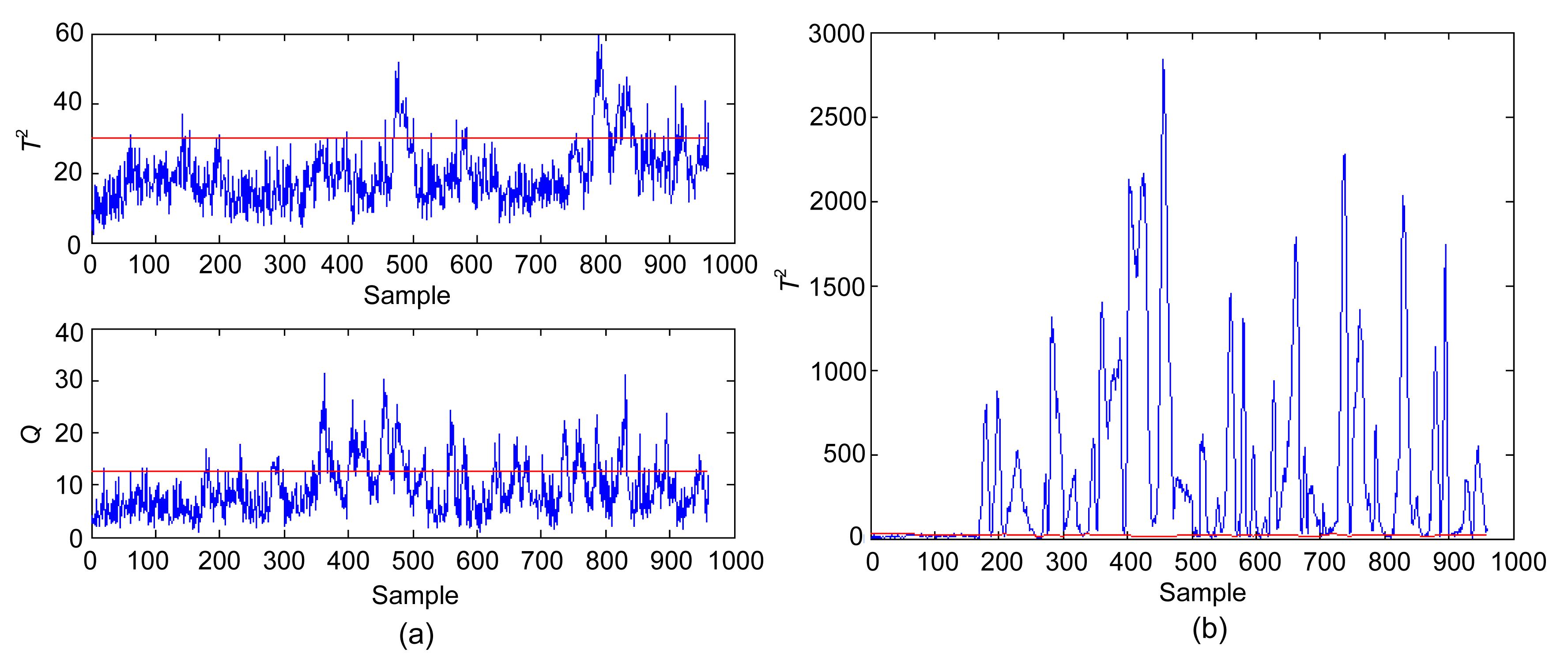
In this study, the time-window length is d=50. The discussion of different window length is illustrated later. The limit of the D index has been selected as 70%, that is, the CPCs can capture 70% of all the variability of the current score matrix. For the normal data set, the monitoring charts for the two methods are shown in Fig. 7. The false alarm rate (Type I error) of normal data are almost at the same degree. The fault detection results of all the 18 faults are listed in Table 3. The conventional PCA-based methods have difficulties in consistently detecting the five faults (Faults 5, 10, 16, 19, and 20), with detection rates of less than 40% in most cases. By contrast, the improved PCA can detect almost all of the 18 faults consistently, with detection rates higher than 80%. The detail fault detection results of Faults 10, 16, and 19 are shown in Figs. 8 to 10, respectively. The results clearly show that the fault detection performance has been greatly improved by the proposed monitoring scheme.
Fig.7 Monitoring results of normal data (a) Conventional PCA; (b) Improved PCA
Table 3
Fault detection rate comparison of conventional PCA and improved PCA (%)
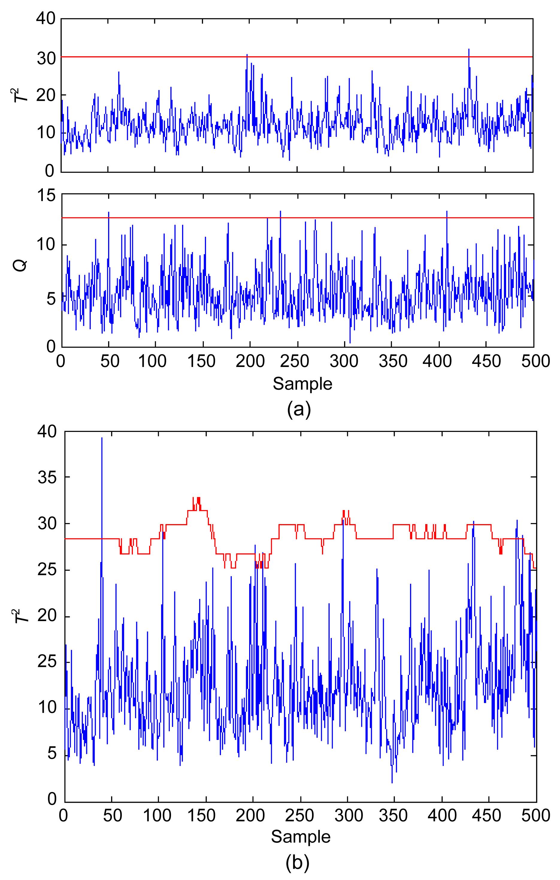
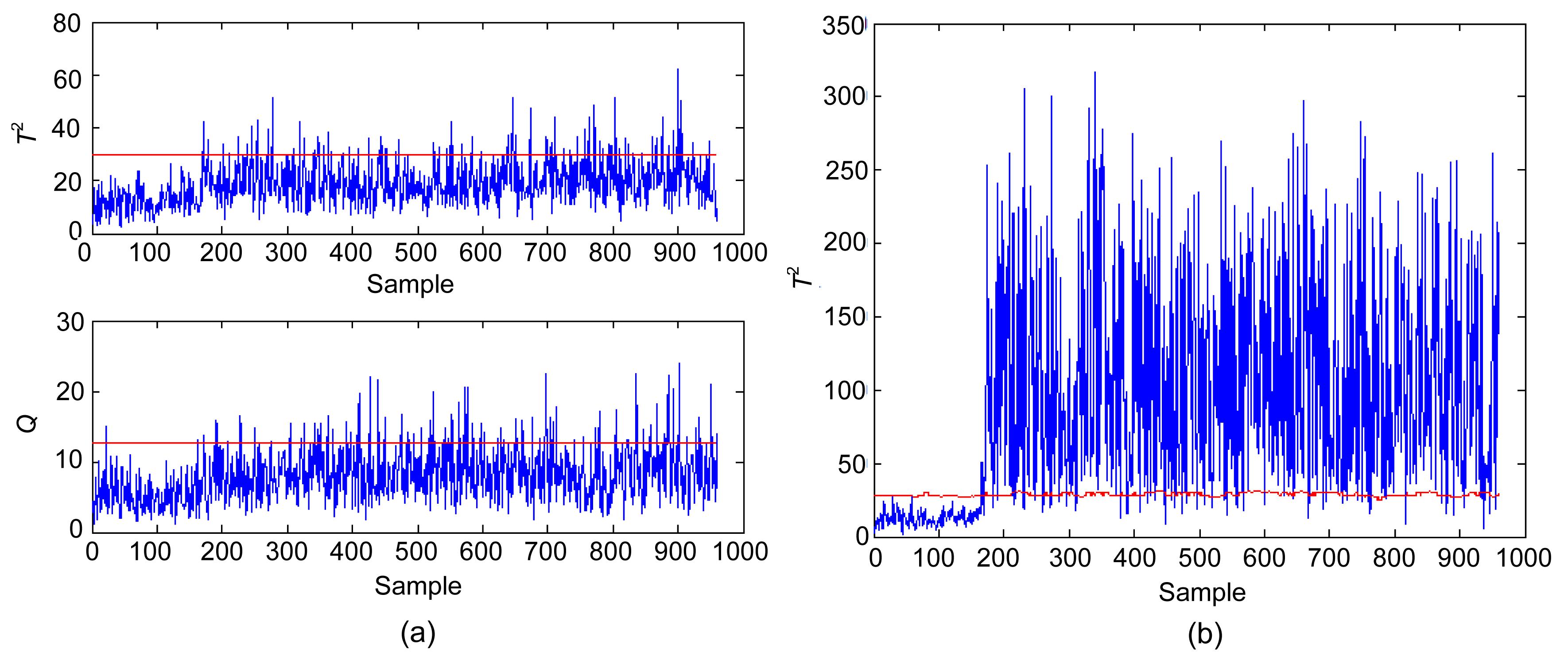
Fig.9 Monitoring results of Fault 16 of the conventional PCA (a) and improved PCA (b)
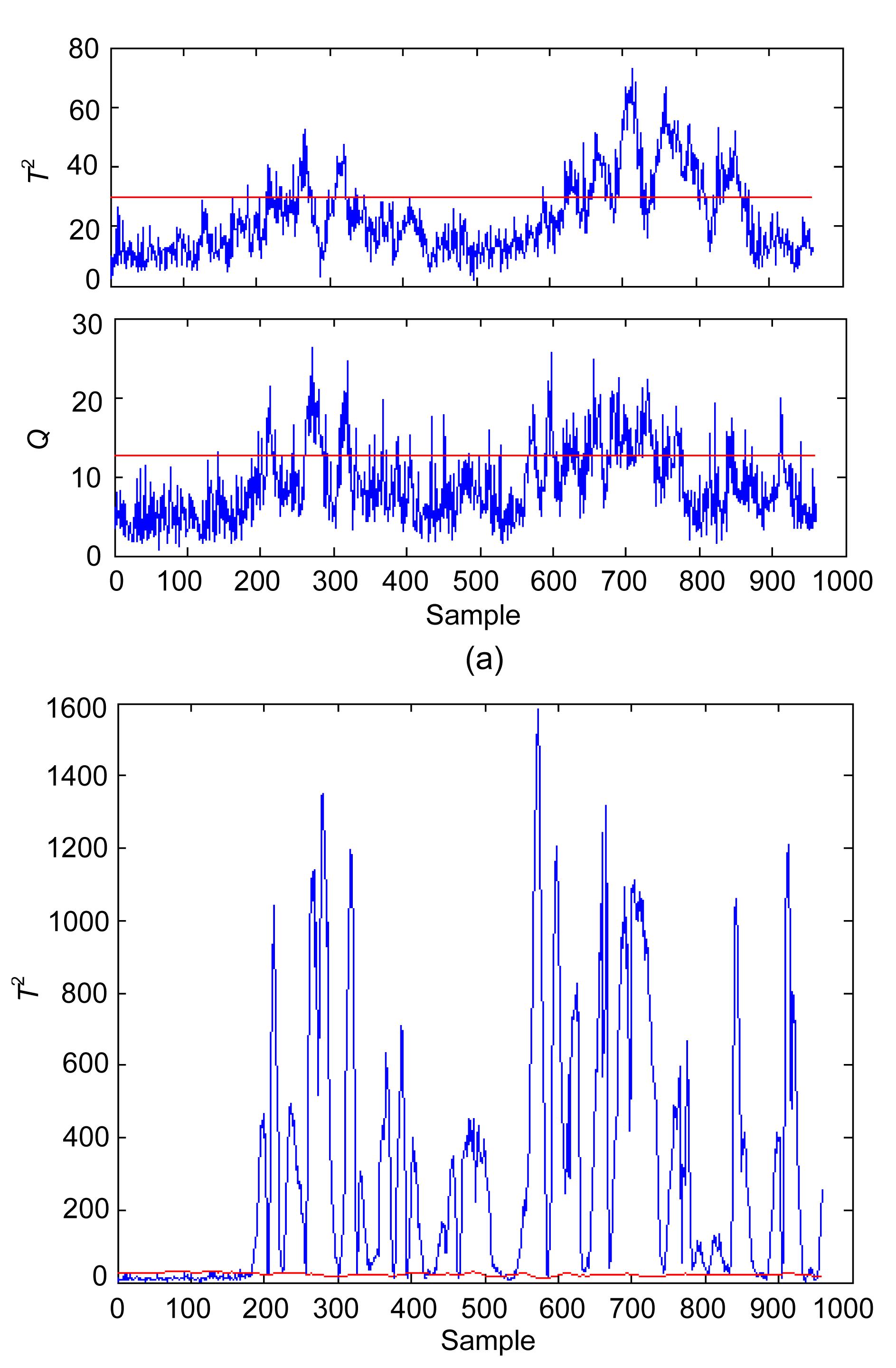
Fig.10 Monitoring results of Fault 19 of the conventional PCA (a) and improved PCA (b)
5. Discussion
5.1. Advantages of utilizing CPCs
Based on the case study described earlier, several points are discussed in this section. First, the feature of the CPCs for statistic T2 is considered. For the PCA-based monitoring method, the number of PCs greatly affects the ability of the fault detection (Tamura and Tsujita, 2007). In addition, a publication of PCA applications indicates that including components with smaller eigenvalues in the PCA model and excluding those with larger eigenvalues can improve the prediction quality (Togkalidou et al., 2001). One advantage of CPCs, as mentioned earlier, is choosing the PCs with significant variation from the reference PCs and excluding those PCs with small variation. This approach focuses on the variation rather than on the variance, thereby leading to better monitoring performance. This advantage is well illustrated by a specific example discussed below.
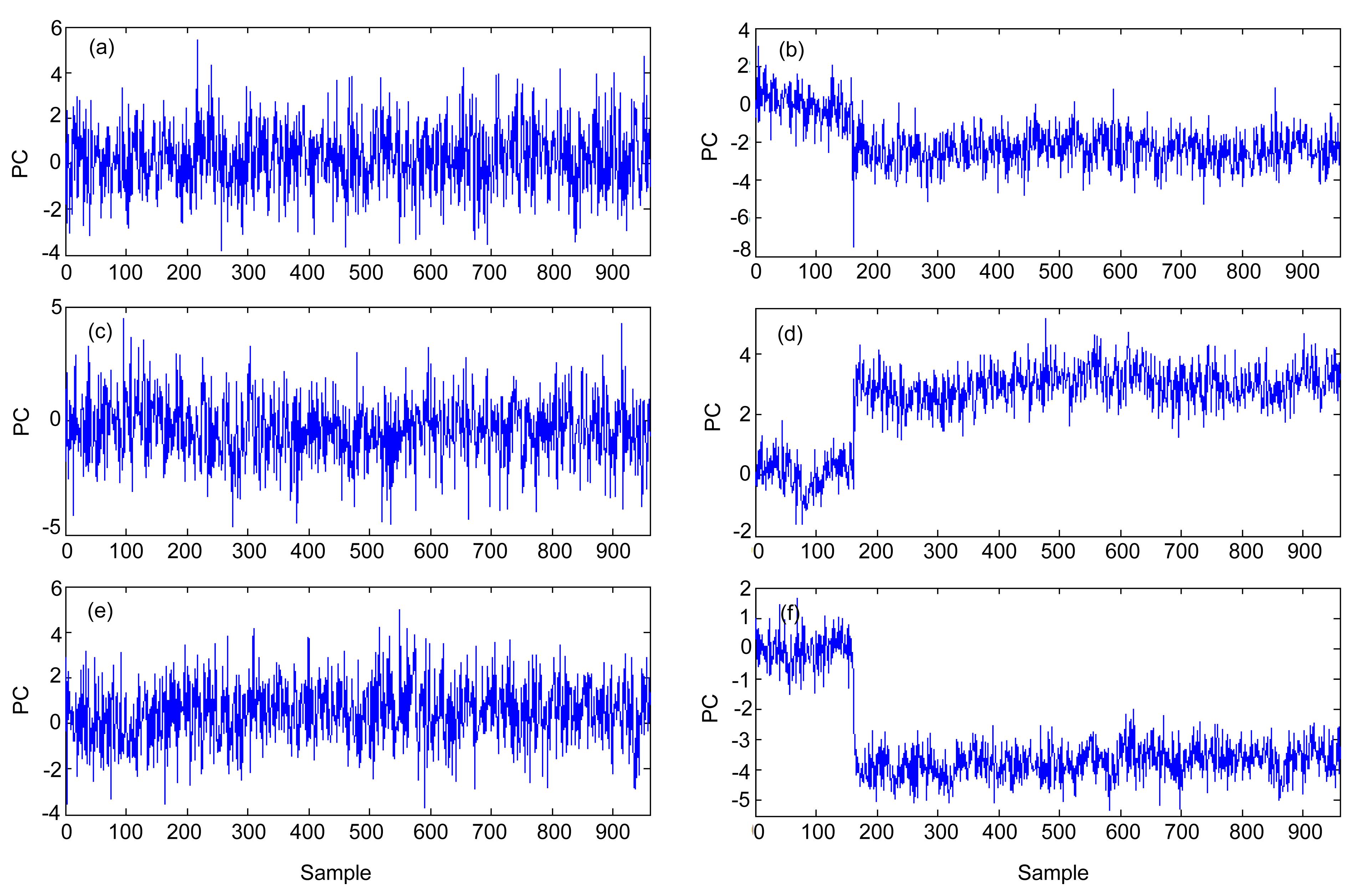
For example, the detection rate of Fault 4 for the improved PCA is higher than that of the conventional PCA. Given that CPCs include the 16th, 21st, and 22nd PCs after the fault occurred, they are ignored by the CPV criterion because they maintain smaller variance compared with the first 14 PCs. Meanwhile, the 4th, 5th, 6th, and other PCs are excluded in CPCs because they present small deviations after the fault occurs. The plots of the above PCs are illustrated in Fig. 11. Retaining PCs with a larger eigenvalue in the PCA model may present a small variability of the abnormal data. As a result, including PCs with smaller eigenvalues for the fault detection can improve the monitoring performance because they show much more significant variation than the other PCs, thereby directly improving the monitoring performance.
Fig.11 Time-series plots of the 4th (a), 5th (b), 6th (c), 16th (d), 21st (e), and 22nd (f) PCs
Second, the false alarm rate of the proposed method is considered. False alarms are expected to increase when numerous PCs are retained because the model may include noise, which yields a large prediction error. Another 500 normal observations are used for analyzing the occurrence frequency of Type I error. The result is shown in Fig. 7. The frequency of Type I error is about 0.4%, almost the same with the conventional PCA. In practice, this significantly low false alarm rates can be neglected. Given the similar variability for all PCs, any PC can be selected as CPC. When we check the number of CPCs, we find that it is less than 14 and lessens when fault occurs. Given that the number of selected PCs is less than that of the CPV criterion, the false alarm rate can be confirmed.
5.2. Detection delay of improved PCA with CPCs
The size of the time-window is a predetermined parameter in the proposed method, which probably results in large delay in the fault detection. The detection delay of the proposed method is discussed in this subsection. Table 4 shows the detection delay result of the 18 faults. Considering an out-of-control value of a statistic can trigger a fault alarm, the fault is indicated only when six consecutive statistic values exceed the control limit to decrease the rate of false alarms (Detroja et al., 2007). The window lengths of d=50, 100, and 150 have little impact on the fault detection delay, and the time delay is not greater than that of the conventional PCA with CPV criterion, and sometimes even better. The index ΔT(i) in Eq. (14) is composed of the correlation and covariance matrices of the current score matrix, which incorporates the 1-norm of the ith column in correlation and covariance matrices. Although the newly added data point is abnormal even if the rest of the data matrix is normal, the degree that the ith element of its score vector changes can be captured by ΔT(i) immediately. Therefore, the detection delay is unlikely to be affected by the size of the time-window.
Table 4
Fault detection delay comparison of the conventional PCA and improve PCA
Fault
Fault detection delay
Conventional PCA
Improved PCA
T2
Q
d=50
d=100
d=150
1
7
2
2
3
3
2
14
34
11
11
12
4
0
0
0
0
0
5
0
1
0
0
0
6
7
0
0
0
0
7
0
0
0
0
0
8
25
19
15
15
15
10
97
48
22
26
28
11
5
5
5
5
6
12
6
2
1
1
2
13
48
40
38
41
43
14
0
0
1
1
1
16
310
21
10
11
11
17
28
21
19
19
19
18
87
83
82
83
84
19
10
–
10
12
12
20
85
86
66
70
71
21
476
256
250
255
255
6. Conclusions
In this work, a novel objective method for determining PCs used for fault detection is developed. Instead of initially selecting several PCs subjectively, the PCs that capture the dominant variability of the current time-window are determined online. Therefore, the selected PCs, termed as CPCs, can capture the dominant process variation dynamically and objectively. Considering the fault detection performance, the novel CPC-based method can be more sensitive to faults.
The proposed method has been applied in the TE process and compared with the conventional PCA to examine its performance. The case study has demonstrated that the improved PCA with CPC-based method detects various faults more efficiently than the conventional PCA method. In particular, the detection delay is superior to the conventional PCA, even with a time-window incorporated into the monitoring scheme. However, the proposed method focuses on the selection of PCs, and the other procedures are similar to the conventional PCA. Therefore, the proposed monitoring procedures suffer from the defects of the conventional PCA and need further investigation.
Appendix: Fast algorithm for updating correlation matrix and covariance matrix
Let the kth data matrix projected onto P with window length d be Rk+1=[tk−d+1, tk−d+2, …, tk]T, similarly, the next data matrix projected onto P would be Tk+1=[tk−d+2, tk−d+3, …, tk+1]T. A two-step adaptation, as shown in Figs. FA1, is used to recursively update covariance matrix S and correlative matrix R.
Fig.A1 Two-step adaptation to construct new data window
Firstly, with eliminating the oldest sample from Tk, the covariance matrix and correlation matrix associated with can be computed recursively. Eqs. (A1) and (A2) describe the variable mean. Eqs. (A3) and (A4) describe the variable variance, while the scaling of the data point is defined in Eq. (A5). , , , , .
A new matrix R* is now introduced to simplify the formation of the equations: .
R*is further derived into: . Then the correlative matrix of Matrix II is expressed as .
Secondly, the next window of selected data (Matrix III) produced by adding the new data point tk+1. With , Sk+1 and Rk+1 associated with Tk+1 are obtained similar to those mentioned above, i.e., , , , , , , where the updated mean vector and the change in the mean vectors are computed from Eqs. (A8) and (A9), and the adaptation of the standard deviations follows from Eqs. (A11) and (A12). The scaling of the new projected data and the updating of covariance and correlation matrix are described in Eqs. (A13), (A10), and (A14), respectively. The adaptation of the standard deviations follows from substituting Eqs. (A2) into (A11) to yield: . In fact, the above two steps can be combined to pro-vide a routine that derives Matrix III directly from Matrix I. Rk+1 is expressed as . Because of the special formulation of covariance matrix, it is easier to update the covariance matrix. The updated Sk+1 is , where b0 is the mean vector of T0 as described above.
References
[1] Alcala, C.F., Qin, S.J., 2010. Reconstruction-based contribution for process monitoring with kernel principal component analysis. Industrial & Engineering Chemistry Research, 49(17):7849-7857.
[2] Chen, X.Y., Yan, X.F., 2012. Using improved self-organizing map for fault diagnosis in chemical industry process. Chemical Engineering Research & Design, in press,:
[3] Chiang, L.H., Russel, E.L., Braatz, R.D., 2001. Fault Detection and Diagnosis in Industrial Systems. Springer,London :
[4] Detroja, K.P., Gudi, R.D., Patwardhan, S.C., 2007. Plant-wide detection and diagnosis using correspondence analysis. Control Engineering Practice, 15(12):1468-1483.
[5] Dunia, R., Qin, S.J., 1998. Joint diagnosis of process and sensor faults using principal component analysis. Control Engineering Practice, 6(4):457-469.
[6] Garcia-Alvarez, D., Fuente, M.J., Sainz, G.G., 2012. Fault detection and isolation in transient states using principal component analysis. Journal of Process Control, 22(3):551-563.
[7] Ge, Z.Q., Song, Z.H., 2008. Batch process monitoring based on multilevel ICA-PCA. Journal of Zhejiang University-SCIENCE A, 9(8):1061-1069.
[8] He, X.B., Wang, W., Yang, Y.P., Yang, Y.H., 2009. Variable-weighted fisher discriminant analysis for process fault diagnosis. Journal of Process Control, 19(6):923-931.
[9] Jackson, J.E., 1991. A Users Guide to Principal Components. John Wiley & Sons,New York :
[11] Kano, M., Nagao, K., Hasebe, S., Hashimoto, I., Ohno, H., Strauss, R., Bakshi, B.R., 2002. Comparison of multivariate statistical process control monitoring methods with applications to the Eastman challenge problem. Computers & Chemical Engineering, 26(2):161-174.
[12] Kourti, T., MacGregor, J.F., 1995. Process analysis, monitoring and diagnosis using multivariate projection methods. Chemometrics & Intelligent Laboratory Systems, 28(1):3-21.
[13] Kresta, J.V., MacGregor, J.F., Marlin, T.E., 1991. Multivariate statistical monitoring of process operating performance. The Canadian Journal of Chemical Engineering, 69(1):35-47.
[14] Ku, W., Storer, R.H., Georgakis, C., 1995. Disturbance detection and isolation by dynamic principal component analysis. Chemometrics & Intelligent Laboratory Systems, 30(1):179-196.
[15] Lee, J.M., Yoo, C.K., Choi, S.W., Vanrolleghem, P.A., Lee, I.B., 2004. Nonlinear process monitoring using kernel principal component analysis. Chemical Engineering Science, 59(1):223-234.
[16] Lee, J.M., Yoo, C.K., Lee, I.B., 2004. Statistical process monitoring with independent component analysis. Journal of Process Control, 14(5):467-485.
[17] Lee, J.M., Qin, S.J., Lee, I.B., 2006. Fault detection and diagnosis based on modified independent component analysis. AIChE Journal, 52(10):3501-3514.
[18] Li, W., Yue, H., Valle, C.S., Qin, S.J., 2000. Recursive PCA for adaptive process monitoring. Journal of Process Control, 10(5):471-486.
[19] Liu, Y.M., Ye, L.B., Zheng, P.Y., Shi, X.R., Hu, B., Liang, J., 2010. Multiscale classification and its application to process monitoring. Journal of Zhejiang University-SCIENCE C (Computers & Electronics), 11(6):425-434.
[20] Lyman, P.R., Georgakist, C., 1995. Plant-wide control of the Tennessee Eastman problem. Computers & Chemical Engineering, 19(3):321-331.
[22] Qin, S.J., 2003. Statistical process monitoring: basics and beyond. Journal of Chemometrics, 17(8-9):480-502.
[23] Russell, E.L., Chiang, L.H., Braatz, R.D., 2000. Fault detection in industrial processes using canonical variate analysis and dynamic principal component analysis. Chemometrics & Intelligent Laboratory Systems, 51(1):81-93.
[24] Stubbs, S., Zhang, J., Morris, J.L., 2012. Fault detection in dynamic processes using a simplified monitoring-specific CVA state space modelling approach. Computers & Chemical Engineering, 41:77-87.
[25] Tamura, M., Tsujita, S., 2007. A study on the number of principal components and sensitivity of fault detection using PCA. Computers & Chemical Engineering, 31(9):1035-1046.
[26] Togkalidou, T., Braatz, R.D., Johnson, B.K., Davidson, O., Andrews, A., 2001. Experimental design and inferential modeling in pharmaceutical crystallization. AIChE Journal, 47(1):160-168.
[27] Valle, S., Li, W., Qin, S.J., 1999. Selection of the number of principal components: the variance of the reconstruction error criterion with a comparison to other methods. Industrial & Engineering Chemistry Research, 38(11):4389-4401.
[28] Wang, J., He, Q.P., 2010. Multivariate statistical process monitoring based on statistics pattern analysis. Industrial Engineering & Chemistry Research, 49(17):7858-7869.
[29] Wang, X., Kruger, U., Irwin, G.W., 2005. Process monitoring approach using fast moving window PCA. Industrial & Engineering Chemistry Research, 44(15):5691-5702.
[30] Wold, S., 1978. Cross-validatory estimation of the number of components in factor and principal components models. Technometrics, 20(4):397-405.
[31] Yoon, S., MacGregor, J., 2001. Fault diagnosis with multivariate statistical models, part I: using steady-state fault signatures. Journal of Process Control, 11(4):387-400.
[32] Yu, J., Qin, S.J., 2008. Multimode process monitoring with Bayesian inference-based finite Gaussian mixture models. AIChE Journal, 54(7):1811-1829.
Open peer comments: Debate/Discuss/Question/Opinion


Open peer comments: Debate/Discuss/Question/Opinion
<1>