Similar articles

Abstract: Preventive maintenance (PM) is very important for the safe, efficient, and reliable operation of mechanical systems. This paper focuses on one of the most challenging tasks for PM: PM scheduling. Two basic principles are integrated to support the PM scheduling of mechanical systems: (1) the cost principle, and (2) the reliability principle. These two PM scheduling principles are regarded as conflicting objectives, and the improved strength Pareto evolutionary algorithm is used to find the Pareto-optimal set within which the best compromise solution can be obtained according to fuzzy set theory. Both conceptual and mathematical models of the proposed multi-principle PM scheduling method are explained, and a case study is provided to illustrate the practical application of the new method.

复杂机械产品多准则预防性维护设计

为复杂机械产品提供满足整机可靠性指标和维护成本指标的预防性维护方案多准则规划方法。 1. 分析了检查、维修、更换等对复杂机械产品零部件工作寿命变化的作用机理；2. 提出了复杂机械产品预防性维护多准则规划方法。 1. 基于非完美维修理论，建立不同模式下零件间工作寿命模型，定义维修效能因子，表征检查、维修、更换对零件寿命的影响；2. 通过求解获得复杂机械产品指定时间区间的预防性维护方案，根据零部件工作寿命，采取维修和更换等预防性维护措施，减少零部件故障的发生。 零部件的预防性维护次数与其故障因子相关；机械产品尤其是复杂机械产品实施定期预防性维护能够减少或消除故障的发生。
预防性维护；多准则优化；工作寿命

1.  Introduction

 Preventive maintenance (PM) is defined as a set of activities aimed at improving the overall reliability and availability of a system (Martorell et al., 2002; Ahmad and Kamaruddin, 2012). Instead of performing maintenance when a system fails, PM aims to reduce the chance of any unexpected failures. Therefore, PM activities are very important for the safety, efficiency, and overall reliability of mechanical products (Tsai et al., 2004).

 During the last few decades, numerous papers have been published on PM modeling and optimization. Levitin and Lisnianski (2000) presented an optimization model for PM scheduling in multi-state series-parallel systems. They considered the cost of unsupplied demand due to failures of components as an important part of the cost effectiveness of PM activities. Cassady and Kutanoglu (2005) developed an integrated mathematical model for a single-machine problem with total weighted expected completion time as the objective function. Their model allows multiple maintenance activities and explicitly captures the risk of not performing maintenance. Bartholomew-Biggs et al. (2006) proposed a new PM formulation which allows the optimal number of occurrences of PM to be determined, along with their optimal timings. The formulation involved the global minimization of a non-smooth performance function. El-Ferik and Ben-Daya (2006) developed a hybrid age-based model for imperfect PM involving maintainable and non-maintainable failure modes. They determined the number of PM actions and the length of PM intervals that minimize the total long-term expected cost per unit time. Tam et al. (2006) analyzed the effect of reliability, budget and breakdown outage cost on the calculation of optimal maintenance intervals. Three models were proposed to calculate optimal maintenance intervals for a multi-component system in a factory subjected to minimum required reliability, maximum allowable budget, and minimum total cost. Alardhi et al. (2007) presented a method for scheduling PM tasks in separate and linked cogeneration plants and satisfying maintenance and production constraints. Lim and Park (2007) proposed a periodic PM policy, by which PM maintains the pattern of the hazard rate unchanged. They evaluated the expected cost rate per unit time based on computing the expected number of failures depending on the hazard rate of the underlying life distribution of the system. Shirmohammadi et al. (2007) presented a method for scheduling the PM of a system subject to random failures, and investigated the decision rule for PM. They defined the time between preventive replacements and cut-off age as decision variables to determine the optimal maintenance policy. Bartholomew et al. (2006) proposed a model in which each action of PM reduces the equipment’s effective age. The optimization process involved minimizing a performance function that allows for the costs of the minimal repairs and eventual system replacement, as well as for the costs of PM during the equipment’s operating lifetime. Chung et al. (2009) proposed a double tier genetic algorithm (GA) approach for multi-factory production networks to keep the system’s reliability at a defined acceptable level and minimize the make-span of the jobs. Harrou et al. (2010) formulated a model of imperfect maintenance optimization for a series-parallel transmission system structure. They improved the availability of a transmission system through selecting the optimal sequence of intervals to perform PM actions. Liao et al. (2010) developed a reliability-centered sequential PM model for a monitored repairable deteriorating system. They supposed that the system’s reliability could be monitored continuously and perfectly, and that whenever it reached a threshold, an imperfect repair must be performed to restore the system. Wang and Lin (2011) proposed an improved particle swarm optimization. The optimal maintenance periods for all components in the system were determined according to their importance for system reliability, to minimize the periodic PM cost for a series-parallel system. Moghaddam and Usher (2011) presented mathematical models and a solution approach to determine the optimal PM schedules for a repairable and maintainable series system with equally-sized periods. Schutz et al. (2011) proposed and modeled periodic and sequential PM policies for a system. The objective of the periodic PM policy was to determine the optimal number of PM checks, and the objective of the sequential PM policy was to determine the optimal number of PM intervals and their duration. Lin and Wang (2012) identified important components and determined their maintenance priorities in a series-parallel system. The optimal maintenance periods of these important components were determined to minimize total maintenance cost, given the allowable worst reliability of a repairable system. Wang and Tsai (2012) established a bi-objective imperfect PM model of a series-parallel system. They developed a unit-cost cumulative reliability expectation measure to evaluate the extent to which maintaining each individual component benefits the total maintenance cost and system reliability over the operational lifetime. Ebrahimipour et al. (2013) developed a multi-objective PM scheduling model in a multiple production line. They defined the reliability of production lines and the costs of maintenance, failure and downtime of a system as multiple objectives, and different thresholds for available manpower, spare part inventory and periods under maintenance were applied.

 From the above, it is evident that the two PM schedule principles presented (cost and reliability) are not unfamiliar to the design community. Furthermore, each principle has been individually adopted by different methods. However, there has been no attempt to integrate these two principles and regard them together as a to-be-solved multi-objective optimization problem. Traditional methods use weighted-sum approaches or require the user to supply a weight vector or a preference vector, before solving the problem. Multiple objectives can become a single objective by use of a weight or preference vector, and the outcome of the optimization process is usually a single optimal solution. To obtain a set of Pareto-optimal solutions for multi-objective optimization, these methods have to be applied many times with different weights or preference vectors. This causes problems in multi-objective optimization and does not emphasize the complete range of the transformed objective uniformly.

 In this paper, we propose a multi-objective evolutionary optimization approach to determine optimal PM schedules. A multi-objective mathematical model is developed to determine a plan for three different PM activities for each component of a mechanical system, and to show how to optimize these activities such that their total cost is minimized and the overall reliability of the mechanical system is maximized simultaneously, over the planning horizon. The improved strength Pareto evolutionary algorithm (ISPEA2) is implemented to find the Pareto-optimal solutions that provide good trade-offs between total cost and overall reliability. Such an approach should be useful for maintenance planners and engineers tasked with the problem of developing recommended maintenance plans for mechanical systems of components. The effectiveness of the proposed approach is illustrated using a numerical example which compares our algorithm with the non-dominated sorted genetic algorithm (NSGA-II) and a generational genetic algorithm (GA).

2.  Multi-principle model of a PM schedule

2.1.  Effects of PM activities on reliability

 Mechanical system performance can be kept as good as possible if great care is taken in PM during its operation. Meanwhile, the life cycle of the mechanical system is extended and its efficiency promoted. To decrease potential risks to the mechanical system or to avoid great economic loss, it is necessary to carry out periodic PM for some important components. PM activities are classified into inspection, maintenance, and replacement. By combining the effects of PM activities on these components, the enhancement in performance of the mechanical system can be calculated.

 We assume that PM scheduling maintenance and replacement activities for each component occur over the period [0, T]. The interval [0, T] is segmented into J discrete intervals. At the end of period j (j=1, 2, …, J), the mechanical system is scheduled for either inspection, maintenance, or replacement. We assume that maintenance or replacement activities in period j reduce the “effective working age” of the mechanical system. Consider a mechanical system of N series subsystems/components (SCs), each subject to deterioration. To account for instantaneous changes in working age and failure rate, we introduce the following notation. Let denote the effective working age of SC _i at the start of period j and denote the effective working age of SC _i at the end of period j. It is clear that: (1) .

 Let Δet _{i , j} denote the change in effective working age of SC _i in period j, the PM activities are carried out at period j. In this study, we assume that either of the three kinds of PM activities occurs at the end of the period. It is clear that: (2) .

2.1.1.  Inspection activity

 In this case, inspection is to be carried out on SC _i in period j. This is often referred to as leaving SC _i in a state of “bad-as-old”. It finds that: (3)

2.1.2.  Maintenance activity

 In this case, SC _i is maintained in period j, which places it into a state somewhere between “good-as -new” and “bad-as-old”. The maintenance activity reduces the effective age of SC _i by a stated percentage of its actual age, that is, (4) , where ε_j is an improvement factor.

 The factor ε_j is similar to that proposed by Jayabalan and Chaudhuri (1992). This factor allows for a variable effect of maintenance on the aging of a mechanical system. When ε_j =0, the effect of maintenance is to return the mechanical system to a state of “good-as-new”. When ε_j =1, maintenance has no effect and the mechanical system remains in a state of “bad-as-old”. The maintenance activity effectively reduces the age of SC _i for the start of the next period. Thus, (5) .

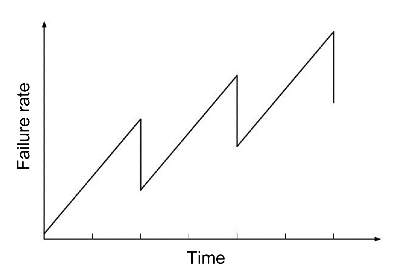
 The rate of occurrence of failure for SC _i is at the end of period j and drops to at the start of period j+1 (Fig. 1).

2.1.3.  Replacement activity

 In this case, SC _i is to be replaced at the end of period j, immediately placing it in a state of “good-as-new”. Its age is effectively returned to time zero. Thus, (6) .

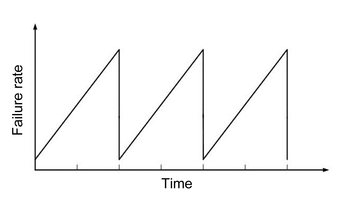
 The rate of occurrence of failure for SC _i instantaneously drops from to h_i (0) (Fig. 2).

2.1.4.  Dynamic reliability of an SC

 Normally, the hazard rate function of any SC can be expressed as a function of reliability. Thus, (7) , where the reliability function R(t) and the hazard rate function h(t) depend on both the intrinsic characteristics of the SC and the extrinsic conditions during use.

 Most failures of mechanical systems can be ascribed to cumulative damage. According to Wang et al. (1996; 1997), each SC _i is assumed to have a rate of occurrence of failure, h_i (t), where t denotes the actual time, and t>0. The Weibull distribution is a reliability-dependent failure rate model which is suitable for describing cumulative failure problems, such as fatigue, wear, corrosion, and thermal creep. In this study, we assume that component failure is given by (8) , where and are the scale and the shape parameters of SC _i , respectively.

 Thus, the reliability of SC _i in period j is given by (9) .

2.2.  Cost of PM activities

 A common problem in planning the PM schedule is to determine the proper PM activities for an SC. To solve this problem, the cost associated with all SC-level maintenance and replacement activities in period j is represented by a function of all the activities carried out during that period.

 If a mechanical system carries a high rate of occurrence of failure through a period, then the mechanical system is at risk of experiencing a high cost of failures. Conversely, a low rate of occurrence of failure in period j should yield a low cost of failure. To account for this, Usher et al. (1998) proposed the computation of the expected number of failures in each period for each SC in a mechanical system. The cost of each failure is cf _i , which in turn is computed as the cost of failures attributable to SC _i in period j as (10) .

 The total cost function can be written as follows: (11) , where ma _i,j is the binary variable of maintenance activity for SC _i in period j. If SC _i at period j is maintained, then ma _i,j =1, otherwise, ma _i,j =0. ra _i,j is the binary variable of replacement activity for SC _i in period j. If SC _i at period j is replaced, then ra _i,j =1, otherwise, ra _i,j =0.

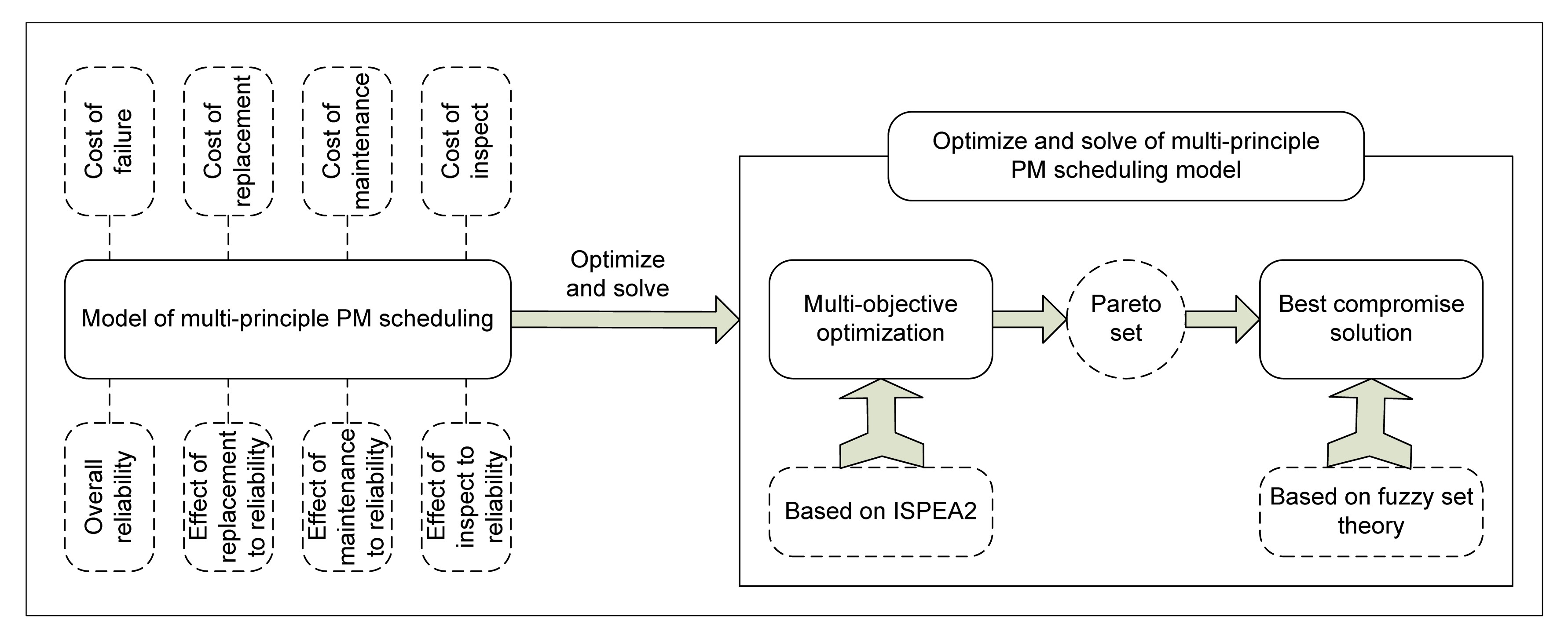
 Fig. 3 illustrates the conceptual modeling of the proposed multi-principle PM scheduling method. The left half of the model indicates that the PM schedule of the mechanical system must simultaneously follow two principles which serve to address different aspects (i.e., the cost of failure, the cost of replacement, and the reliability of an SC) of the mechanical system. This represents the main research problem in this study. The right half of the model indicates the improved multi-objective optimization method (i.e., by treating the two principles as two conflicting objectives) that is used to solve the problem.

2.3.  Multi-objective optimization model of PM schedule

 In the multi-objective optimization model of the PM schedule, we attempt to minimize the total cost and maximize the reliability of the mechanical system. To consider the reliability objective in this model, we take the reliability function for SC _i in the period j as Eq. (9), which can be extended to the reliability function of the mechanical system as (12) .

 The total cost function for the mechanical system is defined as (13) .

 According to the reliability function and the total cost function, the two-objective optimization model of the PM schedule is established as (14) where f' ₁ is the required rate of occurrence of failure and f' ₂ is the given budget. The first set of constraints indicates that only one kind of PM activity occurs in the previous period j. The second set mentions that the initial effective age for each SC is equal to zero. The third set means that the overall rate of occurrence of failure should be kept below f' ₁ and the total cost cannot exceed the given budget f' ₂. The other constraints correspond to the basic assumptions given in Section 2.1.

3.  Multi-objective optimization method based on ISPEA2

3.1.  Presentation of the ISPEA2 algorithm

 Unlike solving a single-objective problem, solving a multi-objective problem will result in a set of “equally good” alternative solutions. Due to the trade-off between objectives, it is impossible to determine which solution is the best in an objective (mathematically sound) manner. Therefore, this set of solutions is also called Pareto, non-dominated, or efficient solutions.

 Once the set of Pareto-optimal solutions is identified, the designer can choose the overall optimum design scheme based on particular requirements and past experience. In the past, many GAs have been prescribed to solve multi-objective optimization problems (Andersson, 2001; Chakraborty et al., 2003; Qiu et al., 2014). Among different multi-objective genetic algorithms (MOGA), the strength Pareto evolutionary algorithm (SPEA2) is commonly regarded as one of the best in terms of search performance. SPEA2 consists of several important operations, such as archiving of individuals with good fitness, density estimation, and fitness assignment (Zitzler et al., 2001). It is commonly believed that SPEA2 can lead to a population with both “precision” and “diversity”. However, the weakness of SPEA2 is that it lacks adequate capability to perform effective crossover. As a result, it can maintain a wide variety of individuals only in the objective space. However, the population distribution in the design variable space is often ignored.

 In contrast, ISPEA2 is a new model of MOGA that features more effective crossover, and results in diverse solutions in both objective and variable spaces. ISPEA2 can be regarded as a particular type of SPEA2 with three additional mechanisms (Kim et al., 2004): (i) neighborhood crossover that allows crossing over individuals located near each other in the objective space; (ii) mating selection that reflects all good solutions within the archive; (iii) application of two archives to maintain the diversity of solutions in both the objective and variable spaces.

3.1.1.  Neighborhood crossover

 Effective crossover is difficult to perform, because the search directions of each parent individual are often completely different. As a result, the search efficiency is always considered a great challenge. Therefore, neighborhood crossover is proposed instead. In neighborhood crossover, individuals within the same search direction are crossed over to generate an offspring that is similar to the parent. Within the sorted population based on arbitrary function values, individuals that are next to each other are defined as neighboring individuals. To avoid crossing over of the same individual, the neighborhood shuffling operation is applied after sorting; neighborhood shuffling counterchanges individuals in the randomized range, which is less than 10% of the population size. The effectiveness of neighborhood crossover in MOGAs has been demonstrated in previous studies (Watanabe et al., 2002). A complete neighborhood crossover consists of three steps:

 Step 1. Sort the population with one of the function values which are altered in each generation.

 Step 2. Perform a neighborhood shuffle for the sorted population.

 Step 3. Select the ith and (i+1)th items as parents, then perform the crossover.

3.1.2.  Mating selection

 In SPEA2, a binary tournament selection is used for mating selection, and individuals with higher fitness are added to the search population of the next generation. By doing so, a population of individuals with high precision can be obtained. However, this will often result in an increase of non-dominated individuals, and in many cases all individuals will become non-dominated at later stages. Alternatively, the use of binary tournament selection often sacrifices the diversity of non-dominated individuals. Therefore, in ISPEA2, an additional copy operation is added to duplicate all archives to the population being searched. This copy operation maintains the diversity of the population and makes the global search possible.

3.2.  Process of the ISPEA2 algorithm

 ISPEA2 creates a design variable archive to store good solutions in the variable space. The purpose is to maintain sufficient diversity in both the objective and variable spaces. Environmental selection of SPEA2 is used to renew the design variable archive. When the number of non-dominated solutions exceeds the archive size, the proximity of individuals is calculated using the Euclidean distance according to the value of the design variables. Based on the proximity result, the archive truncation method is used to reduce the number of individuals. The algorithm flow of ISPEA2 is as follows:

  Procedure: ISPEA2

  Parameters: N, population size; N′, archive size; T, maximum number of generations

  Begin//Initialization: Generate an initial population P ₀ and N random individuals. Create two empty archives: and

  Main loop

  Repeat

 //Fitness assignment: For each individual in P_t , and

 //Environmental selection: From P_t , and creating new archives ,

  If

 The number of individuals in and

  Then

 Archive truncation in the objective space and archive truncation in the variable space

 //Neighborhood crossover and mutation operation: Generate by copying t=t+1

  Until t≥T

 Print all non-dominated solutions in the final population and archive

  End

3.3.  Best compromise solution based on fuzzy set theory

 Fuzzy set theory has been implemented to derive efficiently a candidate trade-off solution for the decision makers (Abido, 2006). Having acquired the final non-dominated set, the proposed approach uses a fuzzy-based mechanism to extract a single non-dominated solution from the trade-off front as the best compromise solution. Due to the imprecise nature of the decision maker’s judgment, the ith objective function of a solution in the non-dominated set F_i , is represented by a membership function μ_i defined as (15) where and are the maximum and minimum values, respectively, of the ith objective function.

 For each non-dominated solution k, the normalized membership function μ^k is calculated as (16) , where M is the number of non-dominated solutions. The best compromise solution is the one having the maximum μ^k . Arranging all solutions in the trade-off front in descending order according to their membership function provides the decision maker with a priority list of non-dominated solutions. This will guide the decision maker in light of the current operating conditions.

4.  Computational results

 A dual-platen mold closing mechanism (DMCM) includes ten SCs: (1) SC₁, head plate, (2) SC₂, gimbals, (3) SC₃, boot, (4) SC₄, drag link, (5) SC₅, lift out attachment, (6) SC₆, steadier, (7) SC₇, base plate, (8) SC₈, die blade, (9) SC₉, oil cylinder, and (10) SC₁₀, carriage.

 To illustrate the models and the proposed solution procedure, the data for parameters of the DMCM for the PM schedule are shown in Table 1. The planning horizon is defined as 1080 d and ci=25 USD is assumed as the fixed cost, f' ₁=0.05 as the required rate of occurrence of failure, and f' ₂=18 000 USD as the given budget for the multi-objective optimization model. Finally, the MATLAB R2008a programming environment is used to develop ISPEA2.




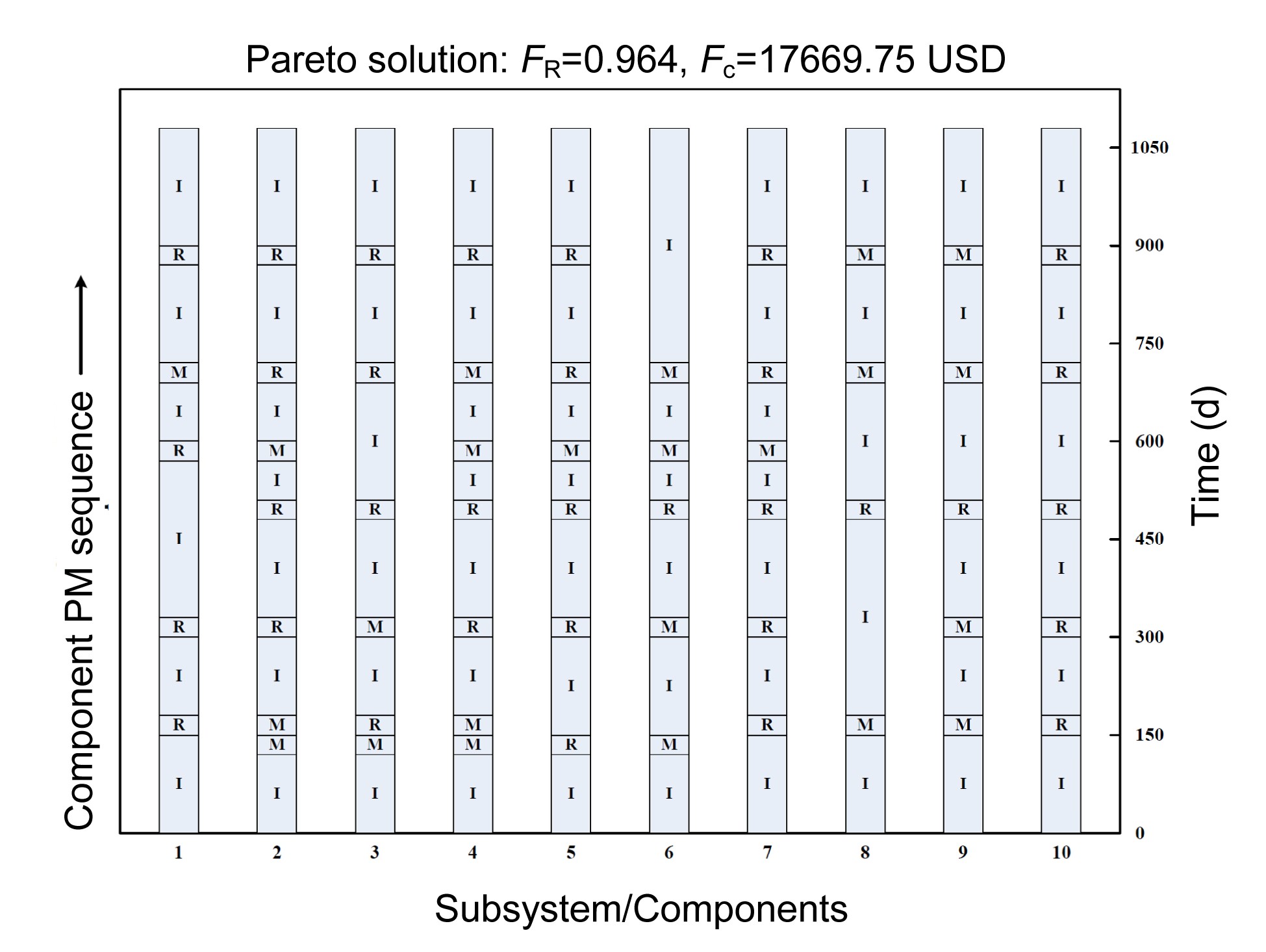
 The optimal PM and replacement schedule for the multi-objective optimization model are presented in Fig. 4. When an SC is maintained, the effective age of that SC drops, based on the value of improvement factors η_i and β_i (Table 1). For example, comparing the variation in the effective age of SC₆ and SC₈ in Fig. 4, we can see that SC₈ is just replaced and no maintenance activity is performed on this SC. On the other hand, SC₆ is just maintained, and replaced only once. This relates to the values of η_i and β_i for each SC. Therefore, it is necessary that SC₈ receives more replacement activities than SC₆ to satisfy the required rate of occurrence of failure.




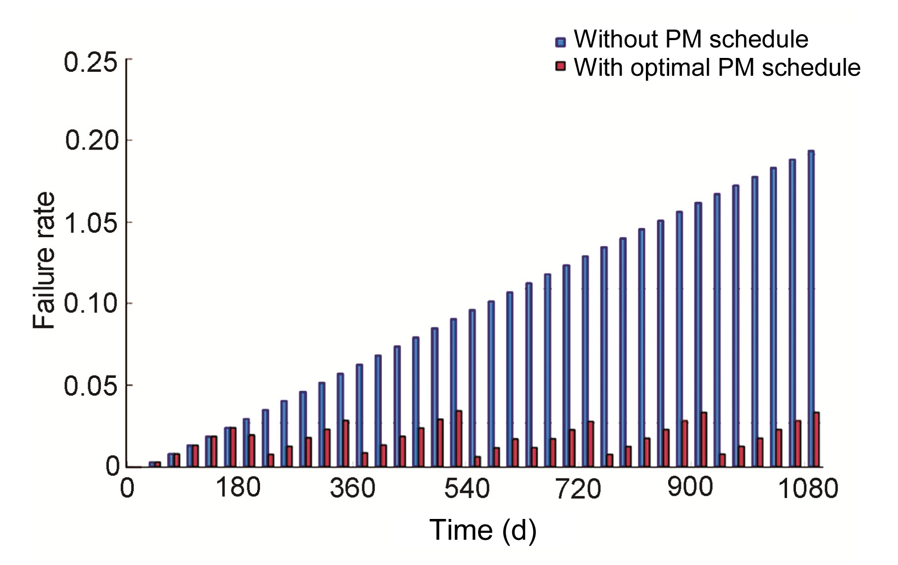
 Fig. 5 shows the rate of occurrence of failure of the DMCM with an optimal PM schedule and without a PM schedule. The rate of occurrence of failure without a PM schedule increases to over 0.05 at 270 d. The rate of occurrence of failure of the DMCM with a PM schedule is lower than 0.05.




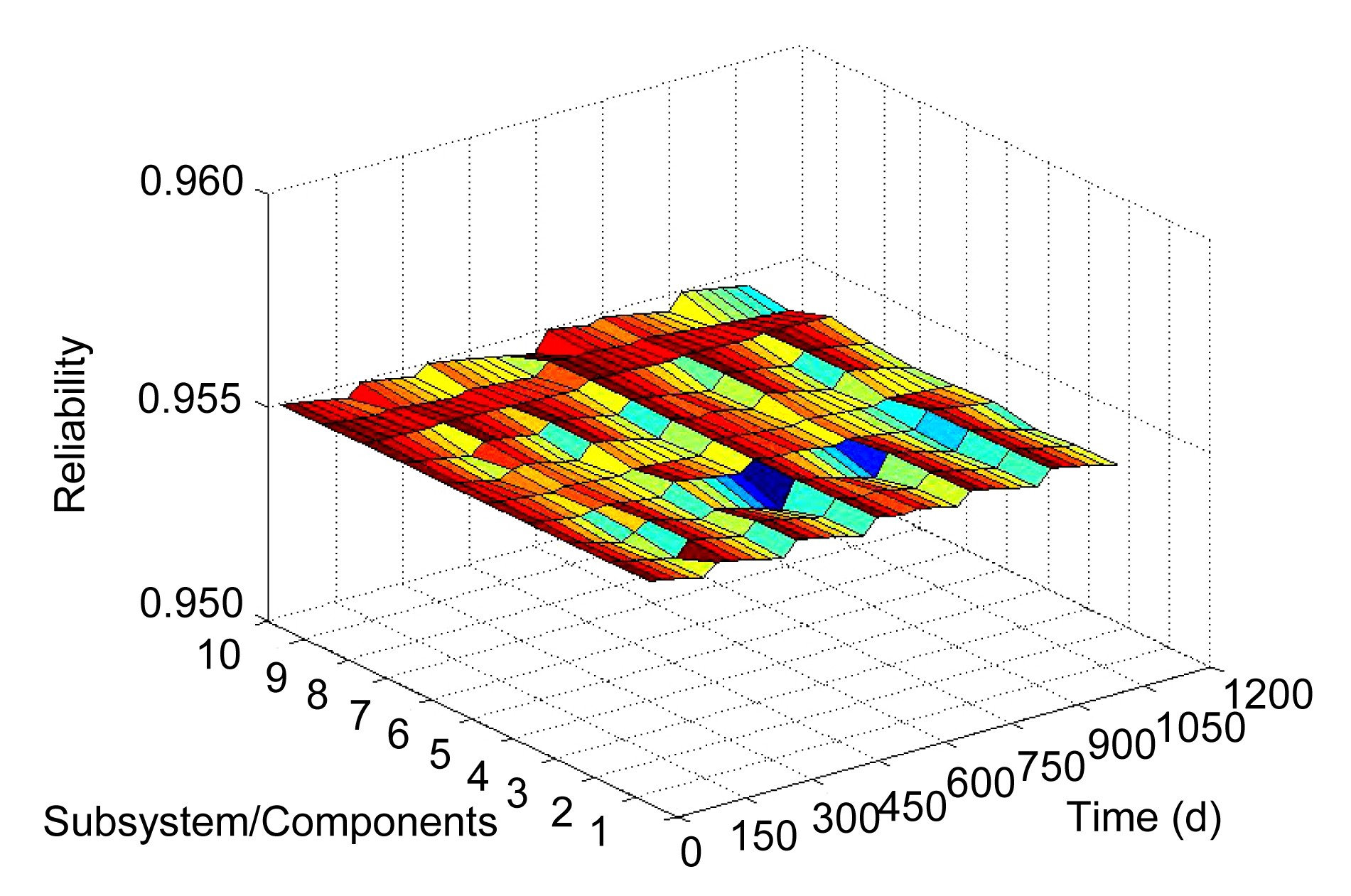
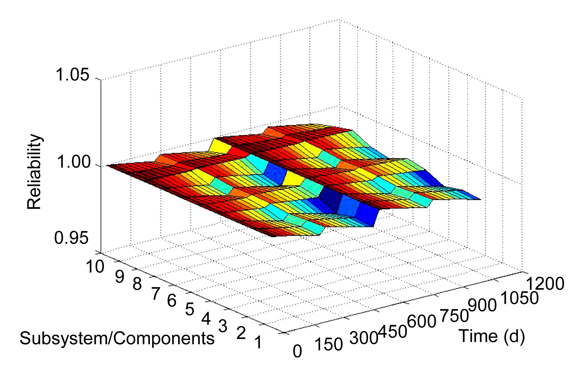
 Fig. 6 illustrates the reliability of the DMCM under the optimal PM schedule and Fig. 7 shows the reliability of SCs of the DMCM under the non-optimal PM schedule. The reliability curve of the optimal PM schedule is smoother and the reliability of each SC is almost the same at each stage in Fig. 6. Therefore, the system under the proposed PM policy is safer than the non-optimal PM schedule considered.







 To test the efficiency and distribution of ISPEA2 solutions, we compared ISPEA2 with NSGA-II and generational GA. To handle multiple objectives using generational GA, the two objective functions are dealt with using a weighted-sum approach. The multi-objective optimization model Eq. (14) is defined as (17)

 A set of values for the weights in the first fitness function was developed to determine the Pareto optimal front. These values were randomly generated in the range of 0 to 1 for both objectives with a condition of ω ₁+ω ₂=1.

 In addition, the parameters for ISPEA2, NSGA-II, and the generational GA were set as presented in Table 2. The MATLAB R2008a programming environment was used to develop ISPEA2, NSGA-II, and generational GA.




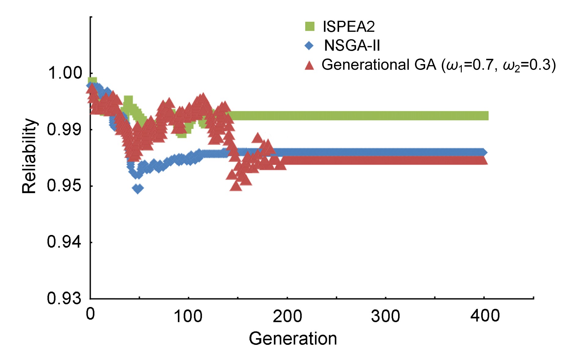
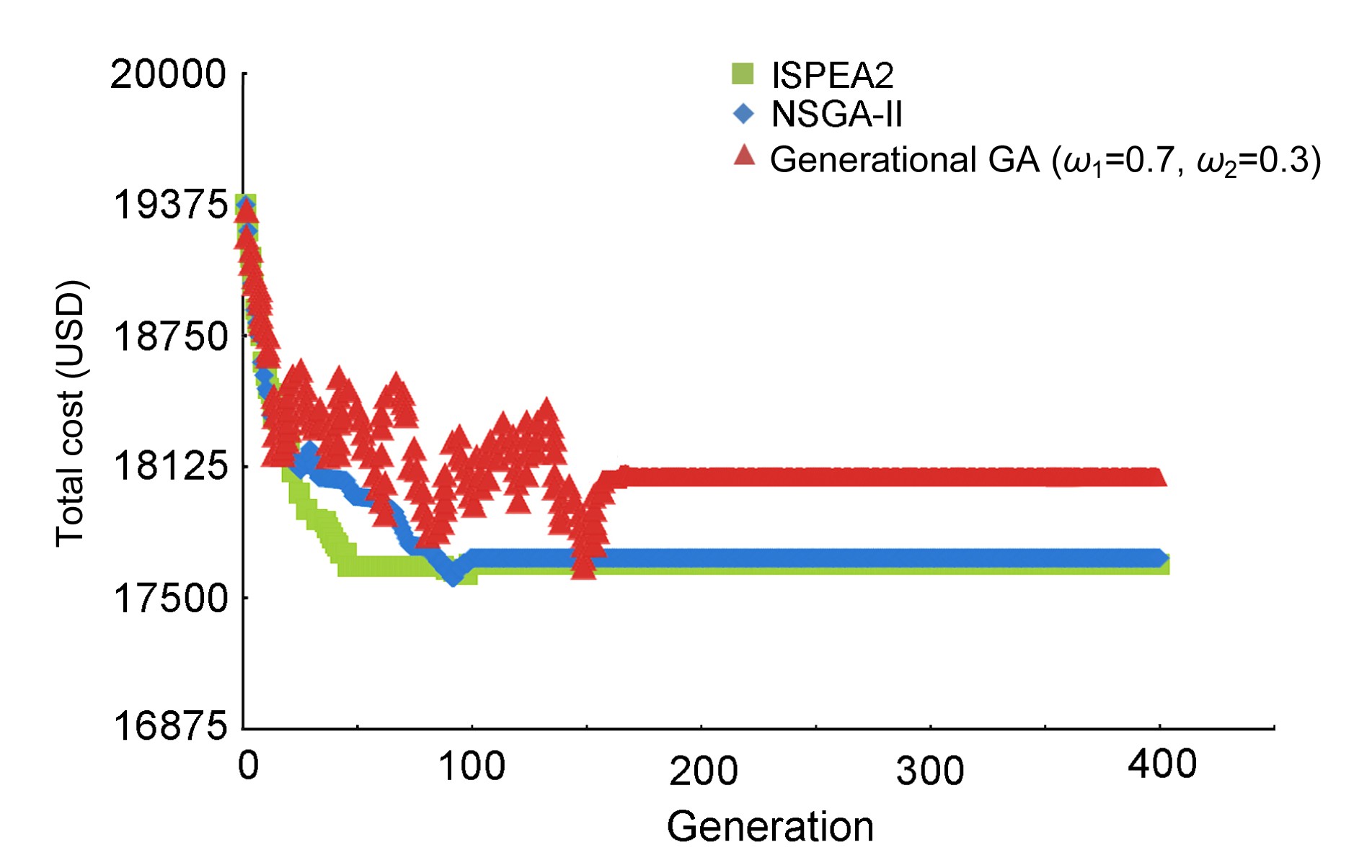
 Figs. 8 and 9 show the reliability and total cost progress of the three algorithms during the generational GA (ω ₁=0.7, ω ₂=0.3). The convergence of the generational GA was not very consistent compared with that of ISPEA2 and NSGA-II with a fitness function Eq. (20). On the other hand, the convergence of ISPEA2 seemed to be faster than that of NSGA-II and generational GA in the first iterations. Although the three algorithms reached almost the same near-optimal solutions at the end, the solutions of ISPEA2 were better than those of the other algorithms. An advantage of ISPEA2 is its ability to search neighborhoods to find both global and local optimum solutions.







 The computational efficiency of the algorithms in terms of CPU time was also examined using a laptop computer (Intel/Core 2, 1.67 GHz, and 2 GB RAM). Table 3 shows the comparisons of ISPEA2, NSGA-II, and generational GA, where the ratio of non-dominated individuals was used to evaluate the accuracy of the obtained solution set. The computational time was less than 3 min for the ISPEA2 and almost 3 min for NSGA-II. ISPEA2 showed better performance than NSGA-II and generational GA in terms of both computing efficiency and accuracy.

5.  Conclusions

 In this paper, we attempted to integrate two principles to support the PM scheduling of mechanical systems: (1) the total cost principle, and (2) the system reliability principle. A multi-objective optimization model is presented, which considers the two principles simultaneously. The multi-objective optimization method is used to find an optimal solution that satisfies all principles. Both the conceptual and mathematical models of the proposed multi-principle PM scheduling method are explained. Furthermore, a case study of PM scheduling of a DMCM is provided to illustrate how this new method can be implemented in practice.

 The proposed new method is expected to deepen understanding of PM of mechanical systems in theory, and to enhance the effectiveness of PM scheduling in practice. The two underlying principles, when treated individually, are not unfamiliar in engineering design. Nevertheless, little effort has been devoted to integrating them as a whole to guide the PM process. In particular, each principle was purposefully selected to address a unique aspect of mechanical systems: total cost and system reliability. From the theoretical development perspective, this paper points out a new direction for addressing the PM of mechanical systems by means of abstracting and integrating fundamental PM scheduling principles. From the practical application perspective, the method presented enables engineers to address multiple aspects of a mechanical system comprehensively (as opposed to separately) and simultaneously (instead of sequentially). Future research will include the application of the proposed method to a more mechanical system than the DMCM.

---

* Project supported by the National Natural Science Foundation of China (Nos. 51205347 and 51322506), the Zhejiang Provincial Natural Science Foundation of China (No. LR14E050003), Project of National Science and Technology Plan (No. 2013IM030500), the Fundamental Research Funds for the Central Universities, the Innovation Foundation of the State Key Laboratory of Fluid Power Transmission and Control, and the Zhejiang University K. P. CHAO’s High Technology Development Foundation, China