Similar articles

Abstract: Modern automotive petrol engine performance is significantly affected by effective tune-up. Current practice of engine tune-up relies on the experience of the automotive engineer, and tune-up is usually done by trial-and-error method and then the vehicle engine is run on the dynamometer to show the actual engine performance. Obviously the current practice involves a large amount of time and money, and then may even fail to tune up the engine optimally because a formal performance model of the engine has not been determined yet. With an emerging technique, support Vector Machines (SVM), the approximate performance model of a petrol vehicle engine can be determined by training the sample engine performance data acquired from the dynamometer. The number of dynamometer tests for an engine tune-up can therefore be reduced because the estimated engine performance model can replace the dynamometer tests to a certain extent. In this paper, the construction, validation and accuracy of the model are discussed. The study showed that the predicted results agree well with the actual test results. To illustrate the significance of the SVM methodology, the results were also compared with that regressed using multilayer feedforward neural networks.

.  INTRODUCTION

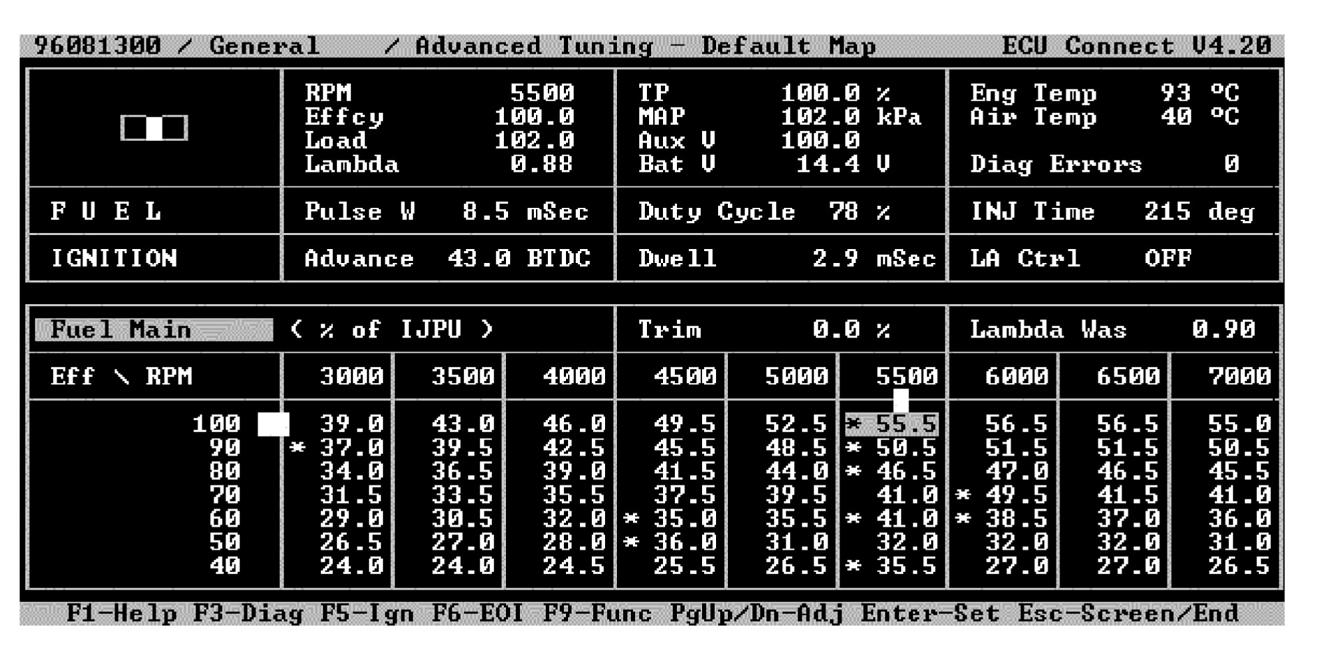
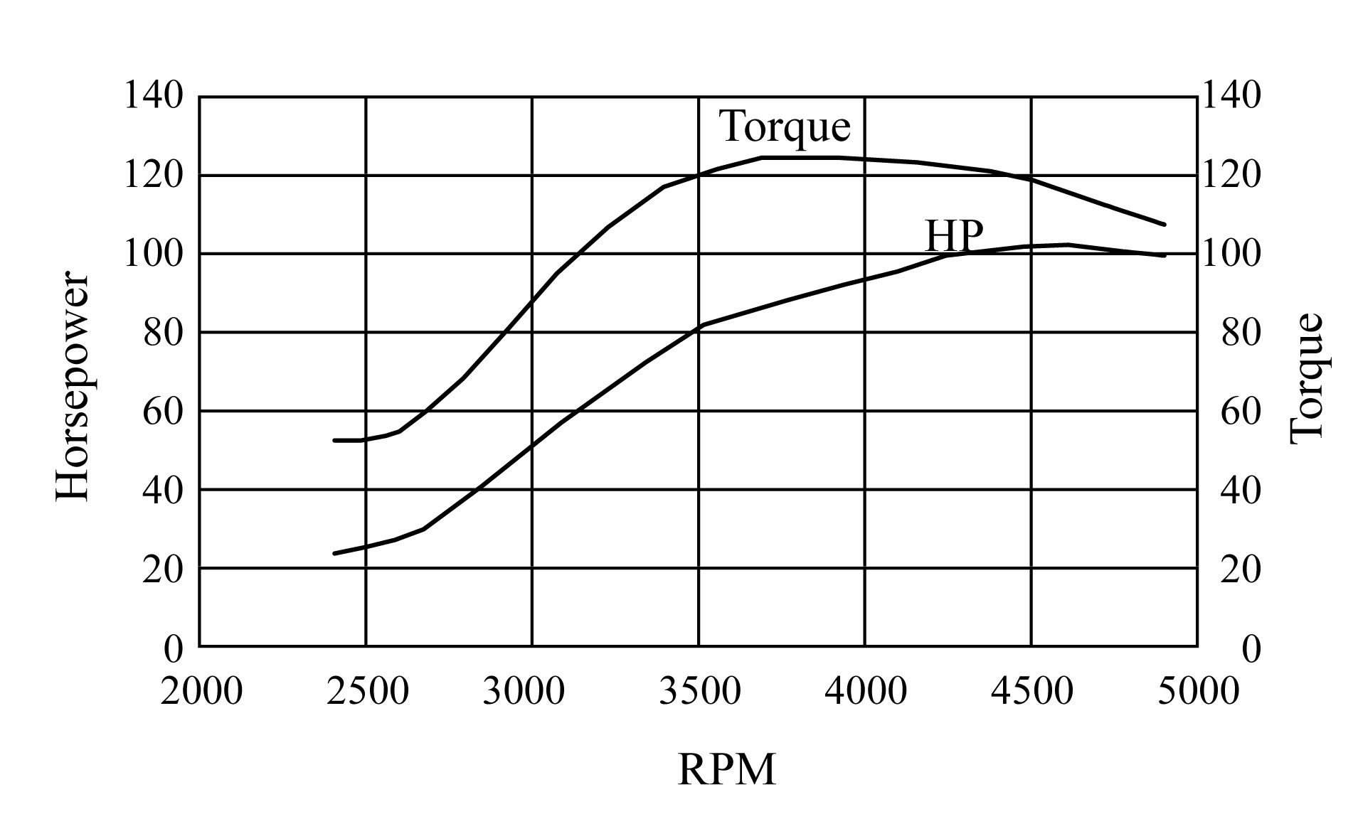
 Modern automotive petrol engines are controlled by the electronic control unit (ECU). The engine performance (such as power output, torque, brake specific fuel-consumption and emission level) is significantly affected by the setup of control parameters in the ECU. Many parameters are stored in the ECU using a look-up table/map (Fig.1). Normally, the car engine performance is obtained through dynamometer tests. An example of performance data on the curve of engine output horsepower and torque against speeds is shown in Fig.2. Traditionally, the setup of ECU is done by the vehicle manufacturer. However, in recent years, programmable ECU and ECU Read Only Memory (ROM) editors have been widely adopted by many passenger cars. These devices allow the non-OEM’s engineers to tune up their engines according to different add-on components and driver’s requirements.







 Current practice of engine tune-up relies on the experience of the automotive engineer who will handle a huge number of combinations of engine control parameters. The relationship between the input and output parameters of a modern car engine is a complex multi-variable nonlinear function, which is very difficult to be determined, because the modern petrol engine is an integration of thermo-fluid, electromechanical and computer control systems. Consequently, engine tune-up is usually done by trial-and-error method. The engineer first guesses an ECU setting based on his/her experience and then stores the setup values in the ECU, and then the engine is run on a dynamometer to test the actual engine performance. If the performance is poor, the engineer adjusts the ECU setting and repeats the procedure until the performance is satisfactory. That is why vehicle manufacturers normally spend many months to tune up an ECU optimally for a new car model. Moreover, the performance function is engine dependent as well. Every engine must undergo similar tune-up procedure.

 By knowing the performance function/model, the automotive engineers can predict if a trial ECU setup is gain or loss. The car engine only requires going through a dynamometer test for verification after estimating a satisfactory parameter setup from the model. Hence the number of unnecessary dynamometer tests for the trail setup can be drastically reduced so as to save a large amount of time and money for testing.

 Recent research papers (Brace, 1998; Traver et al., 1999; Su et al., 2002; Yan et al., 2003; Liu and Fei, 2004) described the use of neutral-networks for modelling the diesel engine emission performance based on experimental data. It is well known that a neural network (Bishop, 1995; Haykin, 1999; Suykens et al.,

 2002) is a universal estimator. It has, however, two main drawbacks (Smola et al., 1996; Schölkopf and Smola, 2002):

 1. The architecture has to be determined a priori or modified while training by heuristic method which results in a not necessarily optimal network structure;

 2. Neural networks can easily be stuck by local minima. Various ways of preventing local minima, like early stopping, weight decay, etc., are employed. However, those methods greatly affect the generalization of the estimated model, i.e., the capacity of handling new input cases.

 Traditional mathematical methods of nonlinear regression (Borowiak, 1989; Ryan, 1996; Seber and Wild, 2003) may be applied to construct the engine performance model. However, an engine setup involves too many parameters and data. Constructing the model in such a high dimensional and nonlinear data space is a very difficult task for traditional regression methods.

 With an emerging technique, Support Vector Machines (SVM) (Cristianini and Shawe-Taylor, 2000; Suykens et al., 2002; Perez-Ruixo et al., 2002; Schölkopf and Smola, 2002), the issues of high dimensionality as well as the previous drawbacks from neural networks are overcome. Using SVM, the regressed engine performance model can be used for precision prediction so that the number of dynamometer tests can be significantly reduced. Moreover, a dynamometer is not always available, particular in the case of on-road fine tune-up. Research on the prediction of modern petrol engine output horsepower and torque subject to various parameter setups in the ECU is still quite rare, so the use of SVM for modelling of engine output horsepower and torque is the first attempt. In this paper, the term, engine performance, refers to the engine output horsepower and torque.

.  SUPPORT VECTOR MACHINES

 SVM is an emerging technique pioneered by Vapnik (Cristianini and Shawe-Taylor, 2000; Schölkopf and Smola, 2002). It is an interdisciplinary field of machine learning, optimization, statistical learning and generalization theory. Basically it can be used for pattern classification and nonlinear regression. SVM considers the application of SVM as a Quadratic Programming (QP) problem of the weights of various factors including regularization factor. Since a QP problem is a convex function, the solution of the QP problem is global (or even unique) instead of a local solution. The advantages of SVM (Smola et al., 1996) as opposed to neural networks are:

 1. The architecture of the system need not be determined before training. Input data of any arbitrary dimension can be treated only linearly regarding the relation of cost to the number of input dimensions;

 2. SVM treats regression as a QP problem of minimizing the data fitting error plus regularization, which produces a global (or even unique) solution having minimum fitting error, while high generalization of the estimated model can also be obtained.

.  SVM formulation for nonlinear regression

 Consider the regression on the dataset, D={(x₁, y₁), …, (x_N, y_N)}, with N data points where x_i∈Rⁿ, y∈R. SVM formulation for nonlinear regression is expressed by the following equation (Gunn, 1998; Cristianini and Shawe-Taylor, 2000; Schölkopf and Smola, 2002; Suykens et al., 2002). such that (1) where, α and α^* are Lagrangian multipliers (Each multiplier is expressed as an N-dimension vector); for 1≤i,j≤N and α_i, α_j, K, kernel function; ε, user pre-defined regularization constant; c, user pre-defined positive real constant for capacity control.

 From the viewpoint of our application, some parameters in Eq.(1) are specified as: N, total number of engine setups (data points); x_i, engine input control parameters in the ith sample data point, i=1,2,…,N (i.e. the ith engine setup); y_i, engine output torque in the ith sample data point.

 (_i and (_i^* are known as support values corresponding to the ith data point, where ith data point means the ith engine setup and output torque. Besides, Radial Basis Function (RBF) with user pre-defined sample variance σ² is chosen as the kernel function because it often yields good result for nonlinear regre-

 ssion (Suykens et al., 2002; Seeger, 2004). After solving Eq.(1) with a commercial optimization package, such as MATLAB and its optimization toolbox, two N-vectors α and α^* are obtained to be the solutions, resulting in the following target nonlinear model: (2) where, b is bias constant; x, new engine input setup with n parameters; σ², user-specified sample variance.

 In order to obtain b, m training data points d_k= <x_k, y_k>∈D, k=1, 2, …, m, are selected, such that their corresponding (_k and (_k^*∈(0, c), i.e., 0<(_k, (_k^*<c. By substituting x_k into Eq.(2) and setting M(x_k)=y_k, a bias b_k can be obtained. Since there are m biases, the optimal bias value b^* is usually obtained by taking the average of b_k as shown in Eq.(3). (3)

.  APPLICATION OF SVM TO PETROL ENGINE MODELLING

 In this application, M(x) in Eq.(2) is the performance function/model of an engine. The issues of use of SVM for this application domain are discussed in the following sub-sections.

.  Schema

 The training dataset is expressed as D={(x_i, y_i)}, i=1 to N. Practically, there are many input control parameters which are also ECU and engine dependent. Moreover, the engine horsepower and torque curves are normally obtained at full-load condition. For demonstrating the SVM methodology, the following common adjustable engine parameters and environmental parameter are selected to be the input (i.e., engine setup) at engine full-load condition.

 x=<I_r, O, t_r, f, J_r, d, a, p> and y=<T_r> where, r is engine speed (rpm) and r={1000, 2000, 3000, …, 8000}; I_r, ignition spark advance at the corresponding engine speed r (degree before top dead centre); O, overall ignition trim (±degree before top dead centre); t_r, fuel injection time at the corresponding engine speed r (millisecond); f, overall fuel trim (±%); J_r, timing for stopping the fuel injection at the corresponding engine speed r (degree before top dead centre); d, ignition dwell time at 15 V (millisecond); a, air temperature (°C); p, fuel pressure (Bar); T_r, engine torque at the corresponding engine speed r (Nm).

 Although the engine speed r is a continuous variable, in practical ECU setup the engineer normally fills the setup parameters for each category of engine speed in a map format. The map usually divides the speed range discretely at 500 intervals as shown in Fig.1, i.e. r={1000, 1500, 2000, 2500, …}. Therefore, it is unnecessary to build a model across all speeds. For this reason, r is manually categorized with a specified interval instead of any integer ranging from 0 to 8500. To simplify our description and experiments, the set of engine speeds is adjusted to {1000, 2000, 3000, …, 8000} at interval of 1000, because the other values of r also follow exactly the same modelling procedure.

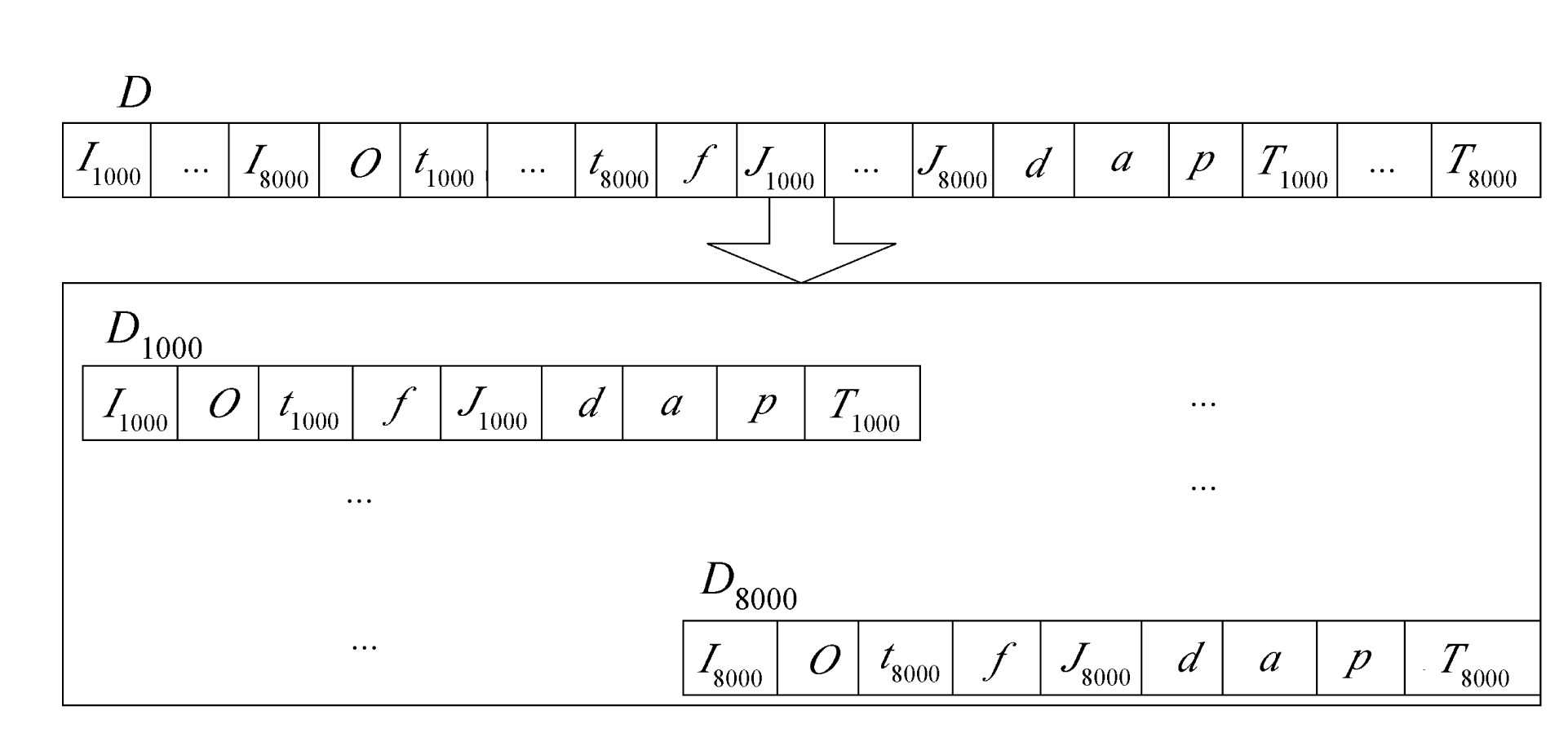
 As some data is engine speed dependent, another notation D_r is used to further specify a dataset containing the data with respect to a specific r. For example, D₁₀₀₀ contains the following parameters: <I₁₀₀₀, O, t₁₀₀₀, f, J₁₀₀₀, d, a, p, T₁₀₀₀>, while D₈₀₀₀ contains <I₈₀₀₀, O, t₈₀₀₀, f, J₈₀₀₀, d, a, p, T₈₀₀₀> (Fig.3).




 Consequently, D is separated into eight subsets namely D₁₀₀₀, D₂₀₀₀, …, D₈₀₀₀. An example of the training data (engine setup) for D₁₀₀₀ is shown in Table 1. For every subset D_r, it is passed to the SVM regression module, Eq.(1), one by one in order to construct eight torque models M_r(x) with respect to engine speed r, i.e. M_r(x)=M_r={M₁₀₀₀, M₂₀₀₀, …, M₈₀₀₀}.




 In this way, the SVM module is run for eight times. At each run, a distinct subset D_r is used as training set to estimate its corresponding torque model. An engine torque against engine speed curve is therefore obtained by fitting a curve that passes through all data points generated by M₁₀₀₀, M₂₀₀₀, …, M₈₀₀₀.

.  DATA SAMPLING AND IMPLMENTATION

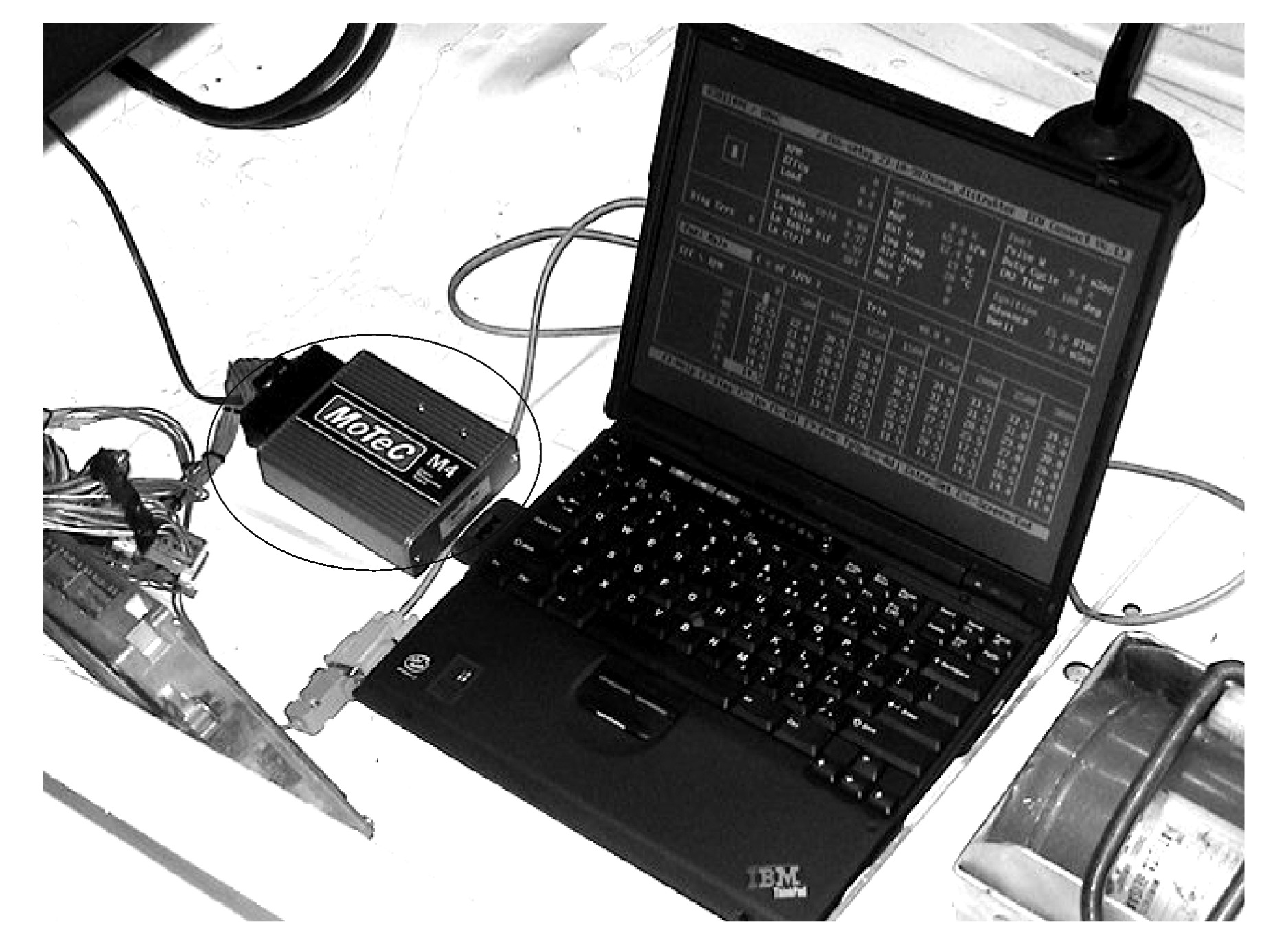
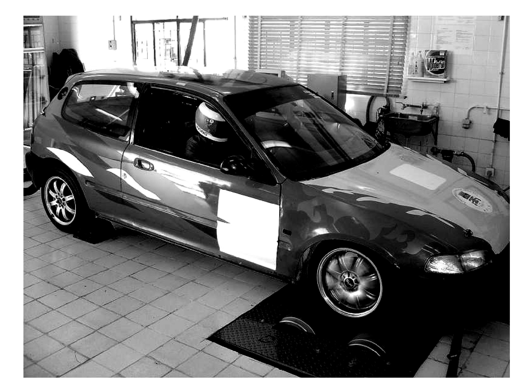
 In practical engine setup, the automotive engineer determines an initial setup, which can basically start the engine, and then the engine is fine-tuned by adjusting the parameters about the initial setup values. Therefore, the input parameters are sampled based on the data points about an initial setup supplied by the engine manufacturer. In our experiment, a sample dataset D of 200 different engine setups along with performance output was acquired from a Honda B16A DOHC engine controlled by a programmable ECU, MoTeC M4 (Fig.4), running on a chassis dynamometer (Fig.5) at wide open throttle. The performance output is only the engine torque against the engine speeds because the horsepower of an engine is calculated using: (4) where, HP is engine horsepower (Hp); r, engine speed (rpm: revolution per minute); T, engine torque (Nm).







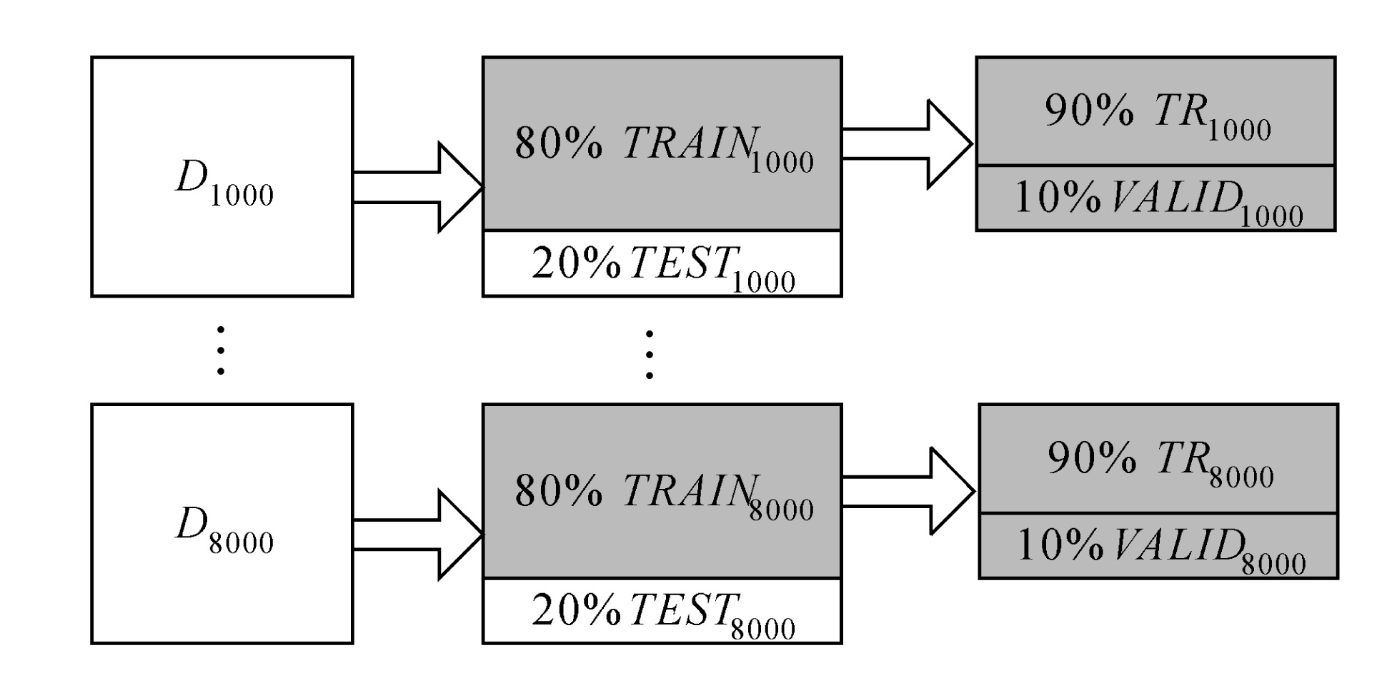
 After collection of sample dataset D, for every data subset D_r⊂D, it is randomly divided into two sets:

 TRAIN_r for training and TEST_r for testing, such that D_r=TRAIN_r∪TEST_r, where TRAIN_r contains 80% of D_r and TEST_r holds the remaining 20% (Fig.6). Then every TRAIN_r is sent to the SVM module for training, which has been implemented using MATLAB 6.5 with its optimization toolbox under MS Windows XP, which is run on a PIII PC with 512 MB RAM. Implementation and other important issues are discussed in the following subsections.

.  Data pre-processing and post-processing

 In order to have a more accurate regression result, the dataset is conventionally normalized before training (Pyle, 1999). This prevents any parameter from dominating the output value. All input and output values must necessarily be normalized within the range [0,1], i.e. unit variance, through the following transformation formula: (5) where, v_min and v_max are the minimum and maximum domain values of the input or output parameter v respectively. For example, v∈[8, 39], v_min=8 and v_max=39. The limits for each input and output parameter of an engine should be predetermined via a number of experiments or expert knowledge or manufacturer data sheets. As all input values are normalized, the output torque value v^* produced by the SVM is not the actual value. It must be re-substituted into Eq.(5) in order to obtain the actual output value v.

.  Error function

 To verify the accuracy of each model of M_r, an error function was established. For a certain model M_r, the corresponding validation error is: (6) where x_i∈Rⁿ is the engine input parameters of ith data point in a test set or a validation set; d_i=<x_i, y_i> represents the ith data point; y_i is the true torque value in the data point d_i; and N is the number of data points in the test set or validation set.

 The error E_r is the root-mean-square of the difference between the true torque value y_i of a test point d_i and its corresponding estimated torque value M_r(x_i). The difference is also divided by the true torque y_i, so that the result is normalized within the range [0, 1]. It can ensure the error E_r also lies in that range. Hence the accuracy rate for each torque model of M_r is calculated using the following formula: (7)

.  Procedures of hyper-parameter values selection

 Eqs.(1) and (2) indicate that the user has to adjust three hyper-parameters (ε, σ, c). Without knowing their best values, all torque models cannot perform well. In order to select the best values for these hyper-parameters, 10-fold cross validation is usually applied (Suykens et al., 2002).

 The 10-fold cross validation means the number of runs is 10 and the training dataset TRAIN_r is further divided into ten parts of data points. In other words, if TRAIN_r has two hundred engine setups, each part contains twenty engine setups.

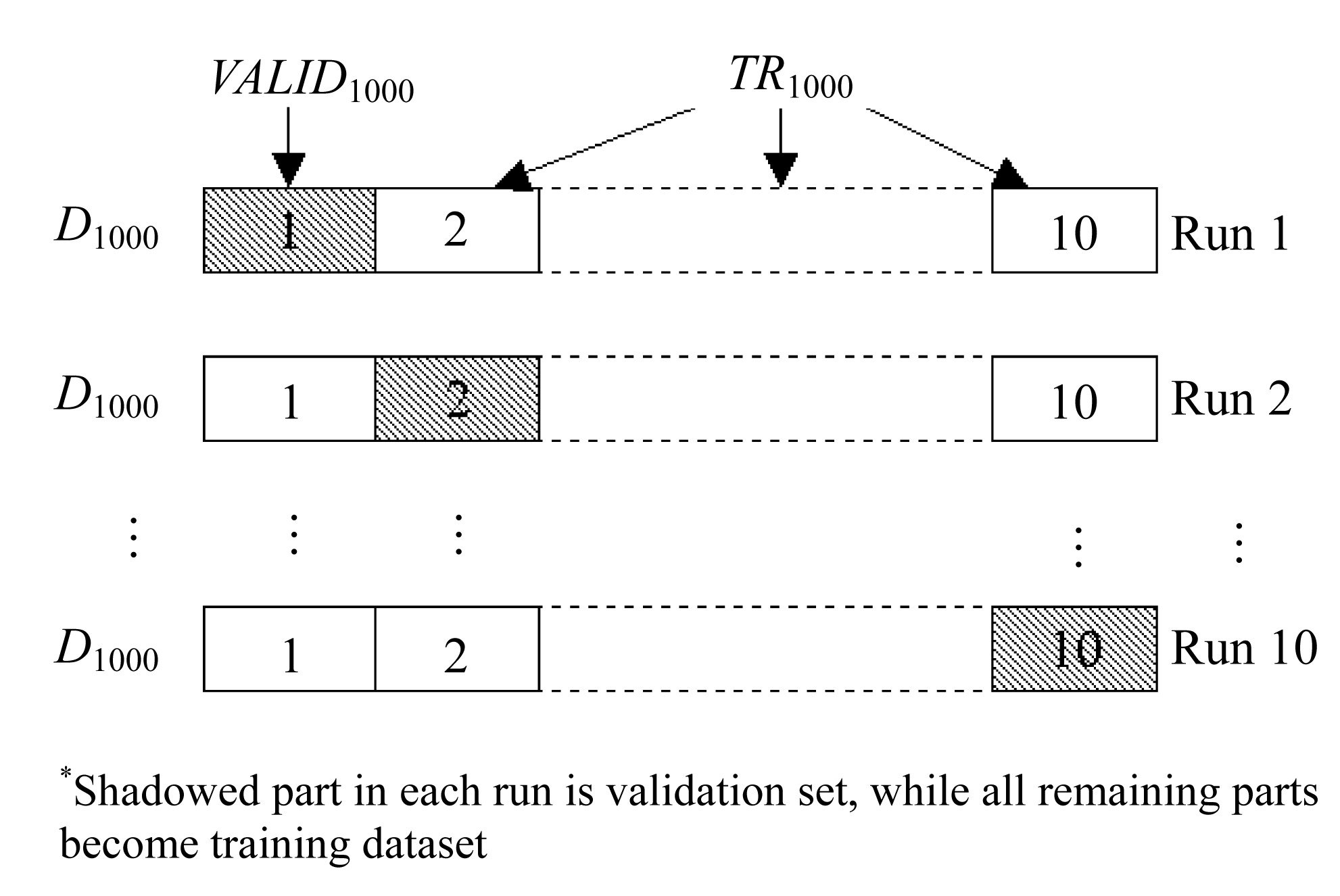
 In each run, one of ten disjoint parts is randomly selected for the purpose of validation. This selected single part is called validation set VALID_r. The remaining nine parts form the training set is denoted as TR_r (Fig.6 and Fig.7). Initially, the values of the hyper-parameters are guessed. With these guessed hyper-parameter values, a torque model is then trained by TR_r, and its corresponding validation error is measured based on VALID_r as well as the error functions in Eq.(6). This procedure is repeated 10 times, each time using different combinations of TR_r and VALID_r. As a result, ten models are produced under the same set of guessed hyper-parameter values. The generalization of the guessed hyper-parameters is assessed by averaging the squared validation errors over the number of runs.




 By guessing different combinations of (ε, σ, c), the best combination of guessed values (i.e., the one with the smallest squared validation error) is chosen because they have the best generalization. Using this combination of hyper-parameters, each target torque model M_r is retrained using all training data TRAIN_r.

 Although 10-fold cross-validation involves 10 different training data and produces 10 different torque models, none of them is the final torque model. The 10 models just have the job of verifying the generalization of hyper-parameters for unseen data. Each torque model is finally produced using the whole training dataset TRAIN_r.

.  Training

 As described in Section 3, the number of combinations of the hyper-parameters is very huge. This is very time-consuming for determining the best combination of the hyper-parameters. In order to simplify our experiment for the SVM methodology demonstration, we assume c=σ=1.0 which are common choices. Hence the remaining hyper-parameter to be found is ε which indicates what the model generalization is. In our case, the value of ε is taken from a range of 0.0 to 0.2 with increment 0.01. That means there are totally 20 values 0.01, 0.02, 0.03, …, 0.2. After applying 10-fold cross validation to a training set TRAIN_r for 20 times, the ( value producing minimum validation error cost for TRAIN_r is chosen to be the best hyper-parameter (_r^*. By repeating this procedure for eight times and all (_r^* values for all TRAIN_r could be determined. Finally, the eight torque models M_r are produced using SVM module based on the corresponding training dataset TRAIN_r and the determined hyper-parameter (_r^*. The biases b^* for different M_r functions can also be easily calculated using Eq.(3).

.  RESULTS

 To illustrate the advantage of SVM regression, the results are compared with those obtained from training a multilayer feedforward neural network (MFN) with backpropagation. Since MFN is a well-known universal estimator, the results from MFN can be considered as a standard benchmark.

.  SVM results

 After obtaining all torque models for an engine, their accuracies are evaluated one by one against their own test sets TEST_r using Eqs.(6) and (7). According to the accuracy obtained in Table 2, the predicted results are in good agreement with the actual test results under their hyper-parameter (_r^*. However, it is believed that the model accuracy could be improved by increasing the number of training data.

.  MFN results

 Eight neural networks NET_r={NET₁₀₀₀, NET₂₀₀₀, …, NET₈₀₀₀} with respect to engine speed r were built based on the same eight sets of training data TRAIN_r=TR_r∪VALID_r. TR_r was actually used for training the corresponding network NET_r whereas VALID_r was used as validation set for early stopping of trainings so as to provide better network generalization.

 Every neural network consists of 8 input neurons (the parameters of an engine setup at a certain engine speed r), one output neuron (the output torque value T_r), and 50 hidden neurons which were just guesses. Normally, 50 hidden neurons can provide enough capability to approximate a highly nonlinear function. The activation function used inside the hidden neurons was Tan-Sigmoid Transfer function while a purely linear filter was employed for the output neuron (Fig.8).




 The training method employed standard backpropagation algorithm (i.e., gradient descent towards the negative direction of the gradient) so that the results of MFN can be considered as a standard. The learning rate of weight update was set to be 0.05. Each network was trained for 300 epochs. The training results of all NET_r are shown in Table 3. The same test sets TEST_r were also chosen so that the accuracy of the models built by SVM and MFN could be compared reasonably. The average accuracy of each NET_r shown in Table 3 was calculated using Eqs.(6) and (7).

.  Discussion of results

 Tables 2 and 3 show that SVM outperforms MFN about 5.56% in overall accuracy under the same test sets TEST_r. In addition, the issues of hyper-parameters and training time were also compared. In SVM, three hyper-parameters ((, (, c) were required for user estimation. They can be guessed using 10-fold cross-validation. In MFN, learning rate and number of hidden neurons are required to be supplied from the users. Surely, these parameters can also be solved by 10-fold cross-validation. However, SVM could often produce better generalization accuracy for unseen examples than MFN as illustrated in Tables 2 and 3.

 Another issue is about the time required for training. With the use of an 800 MHz Pentium III PC with 512 MB RAM, SVM takes about 30 min for training 200 data points of 8 attributes at one time, including the computation for 10-fold cross-validation. There are totally 11 SVM training sessions (10 times for cross-validation, 1 time for final training) for one model. In other words, eight models involve 88 SVM training sessions, so the total training time is about 30×88=2640 min or 44 h. For MFN, an epoch takes about 2 min and each network takes 300 epochs for training. Consequently, it takes about 8×300×2=4800 min or 80 h for eight networks. According to this estimation, SVM training time is only about 55% that of MFN.

.  CONCLUSION

 SVM method was applied to produce a set of torque models for a modern petrol engine with different engine speeds. The models were separately regressed based on eight sets of sample data acquired from an automotive engine through the dynamometer. The prediction models developed are very useful for vehicle fine tune-up because the trial ECU setup can be predicted to be gain or loss before running the vehicle engine on a dynamometer or road test.

 If the engine performance with a test ECU setup can be predicted to be gain, the vehicle engine is then run on a dynamometer for verification. If the engine performance is predicted to be loss, the dynamometer test is unnecessary and another engine setup should be tried. So the prediction models can greatly reduce the number of expensive dynamometer tests, and saves not only the time taken for optimal tune-up, but also the large amount of expenditure on fuel, spare parts, lubricants, etc. It is also believed that the model can let the automotive engineer predict if his/her new engine setup is gain or loss during road tests, where the dynamometer is unavailable.

 Moreover, experiments indicated that the performance and accuracy of the torque models are highly satisfactory. The SVM method outperforms the traditional neural network method by 5.56% in overall accuracy and its training time is approximately 45% less than that using neural-networks. This methodology can be applied to different kinds of vehicle engines.

References

[1] Bishop, C., 1995. Neural Networks for Pattern Recognition, Oxford University Press,:
[2] Borowiak, D., 1989. Model Discrimination for Nonlinear Regression Models, Marcel Dekker,:
[3] Brace, C., 1998. Prediction of Diesel Engine Exhaust Emission using Artificial Neural Networks. , IMechE Seminar S591, Neural Networks in Systems Design, U.K, :
[4] Cristianini, N., Shawe-Taylor, J., 2000. An Introduction to Support Vector Machines and Other Kernel-based Learning Methods, Cambridge University Press,:
[5] Gunn, S., 1998. Support Vector Machines for Classification and Regression. , ISIS Technical Report ISIS-1-98. Image Speech & Intelligent Systems Research Group, University of Southampton, U.K, :
[7] Liu, Z.T., Fei, S.M., 2004. Study of CNG/diesel dual fuel engine’s emissions by means of RBF neural network. J Zhejiang Univ SCI, 5(8):960-965.
[8] Perez-Ruixo, J., Perez-Cruz, F., Figueiras-Vidal, A., Artes-Rodriguez, A., Camps-Valls, G., Soria-Olivas, E., 2002. Cyclosporine concentration prediction using clustering and support vector regression. IEE Electronics Letters, 38:568-570.
[9] Pyle, D., 1999. Data Preparation for Data Mining. , Morgan Kaufmann, :
[10] Ryan, T., 1996. Modern Regression Methods, Wiley-Inter- science,:
[11] Schlkopf, B., Smola, A., 2002. Learning with Kernels: Support Vector Machines, Regularization, Optimization, and Beyond, MIT Press,:
[13] Seeger, M., 2004. Gaussian processes for machine learning. International Journal of Neural Systems, 14(2):1-38.
[14] Smola, A., Burges, C., Drucker, H., 1996. Regression Estimation with Support Vector Learning Machines. Available at. , (Available from:
)http://www.first.gmd.de/ ~smola,:
[15] Su, S., Yan, Z., Yuan, G., 2002. A method for prediction in-cylinder compound combustion emissions. , J Zhejiang Univ SCI, 543-548. (5):543-548.
[16] Suykens, J., Gestel, T., de Brabanter, J., 2002. Least Squares Support Vector Machines. , World Scientific, :
[17] Traver, M., Atkinson, R., Atkinson, C., 1999. Neural Network-based Diesel Engine Emissions Prediction Using In-Cylinder Combustion Pressure. , SAE Paper 1999-01-1532, :
[18] Yan, Z., Zhou, C., Su, S., 2003. Application of neural network in the study of combustion rate of neural gas/diesel dual fuel engine. , J Zhejiang Univ SCI, 170-174. (2):170-174.
Open peer comments: Debate/Discuss/Question/Opinion