ZHANG Sen-lin, LIU Mei-qin. LMI-based approach for global asymptotic stability analysis of continuous BAM neural networks[J]. Journal of Zhejiang University Science A, 2005, 6(1): 32-37.
@article{title="LMI-based approach for global asymptotic stability analysis of continuous BAM neural networks", author="ZHANG Sen-lin, LIU Mei-qin", journal="Journal of Zhejiang University Science A", volume="6", number="1", pages="32-37", year="2005", publisher="Zhejiang University Press & Springer", doi="10.1631/jzus.2005.A0032" }
%0 Journal Article %T LMI-based approach for global asymptotic stability analysis of continuous BAM neural networks %A ZHANG Sen-lin %A LIU Mei-qin %J Journal of Zhejiang University SCIENCE A %V 6 %N 1 %P 32-37 %@ 1673-565X %D 2005 %I Zhejiang University Press & Springer %DOI 10.1631/jzus.2005.A0032
TY - JOUR T1 - LMI-based approach for global asymptotic stability analysis of continuous BAM neural networks A1 - ZHANG Sen-lin A1 - LIU Mei-qin J0 - Journal of Zhejiang University Science A VL - 6 IS - 1 SP - 32 EP - 37 %@ 1673-565X Y1 - 2005 PB - Zhejiang University Press & Springer ER - DOI - 10.1631/jzus.2005.A0032
Abstract: Studies on the stability of the equilibrium points of continuous bidirectional associative memory (BAM) neural network have yielded many useful results. A novel neural network model called standard neural network model (SNNM) is advanced. By using state affine transformation, the BAM neural networks were converted to SNNMs. Some sufficient conditions for the global asymptotic stability of continuous BAM neural networks were derived from studies on the SNNMs’ stability. These conditions were formulated as easily verifiable linear matrix inequalities (LMIs), whose conservativeness is relatively low. The approach proposed extends the known stability results, and can also be applied to other forms of recurrent neural networks (RNNs).
Darkslateblue:Affiliate; Royal Blue:Author; Turquoise:Article
Article Content
. INTRODUCTION
Associative memory model is a kind of commonly used neural network model with the ability of information memory and association. Bidirectional associative memory (BAM) proposed by Kosko (1987) is a generalization of Cohen-Grossberg’s model from single layer to two layers. Since then, researches on BAM had yielded rich results, especially on the stability of neural network models and the improved ones (Liao, 2000; Fu et al., 2000; Cao and Wang, 2002; Zhang et al., 1993; Xu et al., 1992; Jing, 1997). However, all these results were usually in the form of complicated formulas making them difficult for engineering application. As modern robust linear control has a standard representation, called the linear fractional transformation (LFT), for describing models and uncertainty, neural networks may also have a standard representation. We propose that standard neural network model (SNNM) be considered as such a standard representation. By virtue of the similar methods in robust control, most neural network models, of which nonlinear activation functions have bounded output, can be transformed into SNNMs to be analyzed in a unified way. By using Lyapunov method, the global asymptotic stability of the equilibrium points of SNNMs is verified when the equilibrium points locate at the origin. The stable conditions are formulated as linear matrix inequalities (LMIs), which are easily verified and are less conservative. Then, we transform the continuous BAM neural networks into the SNNMs. By solving some LMIs, we know whether the equilibrium points of the continuous BAM neural networks are globally asymptotically stable or not. The approach proposed here will provide a new way for stability analysis and yield some conditions of stability that are better than the previously published results, which is significant for the design and application of the continuous BAM neural networks.
. STATEMENT OF PROBLEMS
The continuous BAM neural network can be described by the following nonlinear differential equations (Jing, 1997): where x(t)=(x1(t), x2(t), …, xn(t))T∈(n and y(t)=(y1(t), y2(t), …, ym(t))T∈(m are state vectors, f(y(t))= (f1(y1(t)), f2(y2(t)), …, fm(ym(t)))T and g(x(t))=(g1(x1(t)), g2(x2(t)), …, gn(xn(t)))T are function vectors, gi (i=1, …, n) and fj (j=1, …, m) are continuously differentiable and monotonically increasing sigmod functions defined from (→(, and fi(0)=gj(0)=0, I=(I1, I2, …, In)T and J=(J1, J2, …, Jm)T are external input vectors, Ii (i=1, …, n) and Jj (j=1, …, m) are constants. W, V are real matrices of n×m, m×n, respectively, A=diag(a1, a2, …, an)>0, B=diag(b1, b2, …, bn)>0.
Let z(t)=(x1(t), x2(t), …, xn(t), y1(t), y2(t), …, ym(t))T∈(n+m, ϕ(z(t))=(g1(x1(t)), g2(x2(t)), …, gn(xn(t)), f1(y1(t)), f2(y2(t)), …, fm(ym(t)))T, then, Eq.(1) can be rewritten as where R=diag(−A, −B) (i=1, …, n+m), , H=(I, J)T. If gi (i=1, …, n), fj (j=1, …, m) are hyperbolic tangents or tanh, ϕi(zi(t)) (i=1, …, n+m) satisfies ϕi(zi(t))∈[−1,1], ϕi(zi(t))/zi(t)∈[0,1] and dϕi(zi(t))/dzi(t) ∈[0, 1].
In this paper, we assume that the training of continuous BAM neural network is finished before we analyze it. Thus, the weights are not changeable in the process of stability analysis. Because there are many detailed discussions on the existence and uniqueness of the equilibrium points of BAM neural networks (Xu et al., 1992; Jing, 1997), we assume that there exists a unique equilibrium point and that it is changed by the different input H. Now the problem under consideration is what are sufficient conditions on weights matrices R and S which guarantee that all the trajectories of system Eq.(2) converge to the (unique) equilibrium point
. STANDARD NEURAL NETWORK MODEL
In robust control, in order to describe models and uncertainty, we transform the system into a standard form called LFT. Similar to the LFT, and referring to the paper written by Moore and Anderson (1968), we can analyze the stability and performance of the neural network by transforming it into a standard form called standard neural network model (SNNM). The SNNM represents a neural network model as the interconnection of a linear dynamic system and static nonlinear operators composed of bounded activation functions. Here, we discuss only the continuous SNNM, since there are similar architecture and results for corresponding discrete-time model (Liu and Zhang, 2003). The continuous SNNM structure is shown in Fig.1. The block Φ is a block diagonal operator composed of nonlinear activation function ϕi(ξi(t)), which will typically be continuous, differentiable, monotonically increasing, slope-restricted, and have bounded output. The matrix N represents a linear mapping between the inputs and outputs of the integrator ∫ (or time delay z−1I in the discrete time case) and the operator Φ. The vectors ξ(t) and ϕ(ξ(t)) are the input and output of the nonlinear operator Φ respectively.
Fig.1 Continuous standard neural network model
If N in Fig.1 is partitioned as where A∈(n×n, B∈(n×L, C∈(L×n, D∈(L×L, x∈(n,
ϕ∈(L, and L∈( is the number of nonlinear activation functions (that is, the total number of neurons in the hidden layers and output layer of the neural network), then, the continuous SNNM can be depicted as a linear difference inclusion (LDI):
The unique equilibrium point of SNNM Eq.(3) is xeq=0. If D=0 and the activation functions satisfy the sector conditions ϕi(ξi(t))/ξi(t)∈[qi, ui], i.e., [ϕi(ξi(t))−qiξi(t)] ˙[ϕi(ξi(t))−uiξi(t)]≤0, i=1, …, L, the following theorem is true.
Theorem 1 The equilibrium point of the continuous SNNM Eq.(3) is asymptotically stable, if there exist a symmetric positive definite matrix P, and diagonal semi-positive definite matrix Λ and τ, such that the following LMI holds: where Q=diag(q1, q2, …, qL),
U=diag(u1, u2, …, uL).
Proof For simplicity, we denote x(t) as x, ξi(t) as ξi, ϕi(ξi(t)) as ϕi, ϕ(ξ(t)) as ϕ. Consider SNNM Eq.(3) and the Lur’e-Postnikov Lyapunov function (Boyd et al., 1994): P>0, λi≥0, thus, ∀x≠0, V(x)>0 and V(x)=0 iff x=0.
The derivative of V(x) with respect to t is
The sector conditions, , can be rewritten as follows: which is equivalent to: where Ci is the ith row of matrix C. Rewriting Eqs.(5) and (6) in matrix notation as follows: where Λ=diag(λ1, λ2, …, λL), T=diag(τ1, τ2, …, τL) and Λ≥0, T≥0.
Although the proof in Theorem 1 is similar to that of the book (Boyd et al., 1994) in page 120, sector boundary in Theorem 1 is any real number and is not limited to [0,1] as in the book (Boyd et al., 1994). So the results in the book (Boyd et al., 1994) are the special case of Theorem 1. When qi=0, ui=1, i=1, …, L, Eq.(4) equals to Eq.(8.6) in the book (Boyd et al., 1994). In the same way, when qi=0, ui=k1, i=1, …, L, Eq.(4) equals to Eq.(9) in the paper (Suykens et al., 1998).
. STABILITY ANALYSIS
To apply Theorem 1 to stability analysis of the continuous BAM neural network, it is necessary to transform the BAM neural network Eq.(2) to the SNNM Eq.(3). We move the equilibrium point to the origin and have
If zeq is the unique equilibrium point of system Eq.(7), it satisfies
0=Rzeq+Sϕ(zeq)+H
Taking the affine transformation z′(t)=z(t)−zeq to system Eq.(7), we get
System Eq.(8) has the same form as system Eq.(7), but the equilibrium point of this system is at the origin. The components of the nonlinear activation function η ηi(σi(t))=ϕi(σi(t)+zeqi)−ϕi(zeqi) (i=1, …, n+m) are different if zeqi are different. But ηi keeps some properties of ϕi. In system Eq.(8), if ϕi is taken to be hyperbolic tangent, or tanh, ηi(σi(t))=tanh(σi(t)+zeqi)− tanh(zeqi). If zeq=0, the sectors for each function ηi are [0, 1]. When zeq≠0, their sector is the subset of the former.
Let φi(s)=tanh(s+zeqi)−tanh(zeqi), the upper bounds of the sectors can be calculated by
ui= max{φi(s)/s:s≠0}, U=diag{ui}.
According to Eq.(7) and Theorem 1 in Xu et al.(1992), it follows that the absolute values of each coordinate of the vector Rz(t)+Sϕ(ξ(t)) are less or equal to 1 if system Eq.(7) has an asymptotically stable equilibrium point. Therefore one can obtain |ξi|≤1+|Hi|=ri for all i=1, …, n+m. Thus, |s+zeqi|≤ri, |zeqi|<ri. The lower bounds for the sectors can be established by the following Lemma 1.
Lemma 1 If |s+zeqi|≤ri, then φi(s)/s≥qi=(tanh(ri) −tanh(|zeqi|))/(ri−|zeqi|), Q=diag{qi}[if |zeqi|=ri, qi =d(tanh(s))/ds (s=ri)].
The proof of Lemma 1 can be referred to the proof of the Lemma 1 in the paper of Barabanov and Prokhorov (2002).
Therefore, system Eq.(8) is transformed into the form of SNNM (3), where A=R, B=S, C=E(n+m)×(n+m), D=0, L=n+m. Also, the nonlinear activation function ηi(σi(k)) satisfies sector condition [qi, ui]. Thereby, we can use Theorem 1 to analyze the global asymptotic stability for system Eq.(8) [equivalently, system Eq.(1)].
Here, we summarize the steps of our approach for stability analysis of the continuous BAM neural network Eq.(1).
1. The continuous BAM neural network Eq.(1) should be transformed into the form of system Eq.(7).
2. It is necessary to find an equilibrium point zeq of system Eq.(7). If the stationary point of the BAM neural network Eq.(1) is determined during training, it becomes an equilibrium point of system Eq.(7). Otherwise, one can use a simple procedure of calculating a few trajectories of the system until the state vector converges to the equilibrium point.
3. The state vector should be shifted in such a way that the equilibrium point of system Eq.(7) moves to the origin. Thus, system EQ.(7) is changed to system Eq.(8). The nonlinear activation functions should be altered correspondingly.
4. For each transformed transfer function [which has a form φi(s)=tanh(s+zeqi)−tanh(zeqi)] it is necessary to calculate the upper bound of a sector in which the plot of this function lies. It may be done using the MATLAB’s function fiminbnd for calculating the minima of −φi(s)/s, and then the upper bound of φi(s)/s. We can use Lemma 1 to find the lower bound of φi(s)/s. Therefore we get Q and U.
5. The MATLAB LMI Toolbox (Gahinet et al., 1995) can be used to solve the LMI Eq.(4) to confirm if the BAM neural network (1) is stable. Note that: if the LMI Eq.(4) has no feasible solutions, the stability of the BAM neural network Eq.(1) cannot be judged. We may analyze its stability by other complicated method.
. AN EXAMPLE
Now we analyze the global asymptotic stability of a continuous BAM neural network with 4 neurons. The dynamic equations can be written as:
The connection weights of system Eq.(9) satisfy Theorem 1 in the paper (Xu et al., 1992), so system Eq.(9) has an asymptotically stable equilibrium point. Transform system Eq.(9) into the form of system Eq.(7), where
z(t)=(x1(t), x2(t), y1(t), y2(t))T,
R=diag(−1.1, −1.2, −1.3, −1.4),
H=(1.0, −1.0, 2.0, −2.0)T,
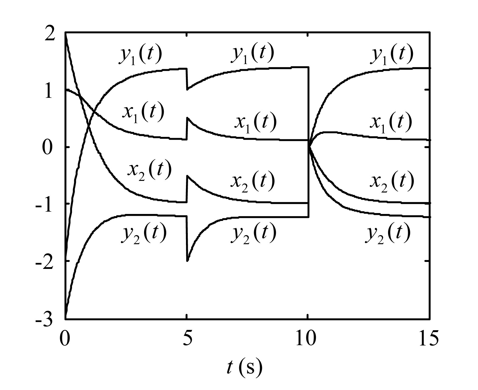
S= then the unique equilibrium point is located at zeq=(0.1175, −0.9906, 1.3786, −1.2226)T. After calculating the bounds of a sector U=diag{0.9966, 0.8188, 0.7165, 0.7565}, Q=diag{0.4500, 0.2045, 0.0706, 0.0870}, we invoke the LMI solver of MATLAB LMI Toolbox (Gahinet et al., 1995) to solve the LMI Eq.(4). The solver returns the following feasible solutions: P is positive definite matrix. Λ and τ are all diagonal and positive definite matrices. From Theorem 1, we conclude that the equilibrium point zeq is globally asymptotically stable. The state trajectory is shown in Fig.2. Our result is independent of the initial value. Theorem 1, Theorem 2 and Theorem 3 in Xu et al.(1992) and Theorem 2, Theorem 3 and Theorem 4 in Jing (1997) can only be used to analyze the locally asymptotic stability, however, if we can find the parameter P, Λ and τ which satisfy some LMIs, it is easy to judge the global asymptotic stability of the BAM neural networks.
Fig.2 The state trajectories of the continuous BAM neural network with 4 neurons x1(t), x2(t), y1(t) and y2(t) are initialized arbitrarily at t=0 s, t=5 s and t=10 s respectively
. CONCLUSION AND FUTURE DIRECTIONS
Although there are many researches on the asymptotic stability of the continuous BAM neural networks, in this paper we proposed a novel neural network model called standard neural network model (SNNM) which simplifies the procedure for analyzing the stability of the BAM neural network. We transform the continuous BAM neural network into SNNM form. Theorem 1 can be used to judge the global asymptotic stability of SNNM and then of the continuous BAM neural network. Our approach is easily verifiable, less conservative, meaningful to the design and application of the BAM neural network, and can be applied to other forms of neural networks, such as BAM neural networks with delays. Since Theorem 1 gives only the sufficient condition of global asymptotic stability for SNNM, if we could not get the feasible solutions of the LMI, we could not judge whether the system is unstable or not. Reducing the intensity of the hetero-association or the sector, we may get the feasible solutions of the LMI. However, it would also weaken the performance of the continuous BAM neural networks. A direction of our research is how to achieve a reasonable compromise between stability and performance of the BAM neural networks. On the other hand, our approach is only
restricted to the sector condition. For particular activation functions (e.g. tanh), however, we could mitigate the conservatism for the stable conditions by using their other properties (e.g. restricted slope). It is another direction we will research in future.
[1] Barabanov, N.E., Prokhorov, D.V., 2002. Stability analysis of discrete-time recurrent neural networks. IEEE Trans on Neural Networks, 13(2):292-303.
[2] Boyd, S.P., Ghaoui, L.E., Feron, E., 1994. Linear Matrix Inequalities in System and Control Theory. , SIAM, Philadelphia, PA, 23-24. :23-24.
[3] Cao, J.D., Wang, L., 2002. Exponential stability and periodic oscillatory solution in BAM networks with delays. IEEE Trans on Neural Networks, 13(2):457-463.
[4] Fu, Y.L., Zhao, Y., Fan, Z., Liao, X.X., 2000. Bidirectional associative memory model with delays. J Huazhong Univ of Sci & Tech, (in Chinese),28(7):80-82.
[5] Gahinet, P., Nemirovski, A., Laub, A.J., 1995. LMI Control Toolbox. , The Math Works Inc., Natick, MA, :
[6] Jing, C., 1997. Asymptotic stability of continuous bidirectional associative memory networks. Pattern Recognition and Artificial Intelligence, (in Chinese),10(1):81-86.
[8] Liao, X.X., 2000. Theory and Application of Stability for Dynamical Systems, (in Chinese), National Defence Industrial Press, Beijing, China,:186-214.
[9] Liu, M.Q., Zhang, S.L., 2003. Stability analysis of a class of discrete-time recurrent neural networks: an LMI approach. Journal of Zhejiang University (Engineering Science), (in Chinese),37(1):19-23.
[10] Moore, J.B., Anderson, B.D.O., 1968. A generalization of the Popov criterion. Journal of the Franklin Institute, 285(6):488-492.
[11] Suykens, J.A.K., Vandewalle, J., Moor, B.D., 1998. An absolute stability criterion for the Lur’e problem with sector and slope restricted nonlinearities. IEEE Trans on Circuits and Systems-I, 45(9):1007-1009.
[12] Xu, B.Z., Zhang, B.L., Kwong, C.P., 1992. Asymptotic Stability Analysis of Continuous Bidirectional Associative Memory Networks. , IEEE International Conference on Systems Engineering, Kobe, Japan, 572-575. :572-575.
[13] Zhang, B.L., Xu, B.Z., Kwong, P.K., 1993. Performance analysis of the bidirectional associative memory and an improved model from the matched-filtering viewpoint. IEEE Trans on Neural Networks, 4(5):864-872.
Open peer comments: Debate/Discuss/Question/Opinion


Open peer comments: Debate/Discuss/Question/Opinion
<1>