Similar articles

Abstract: In this paper, a model named fictitious soil pile was introduced to solve the boundary coupled problem at the pile tip. In the model, the soil column between pile tip and bedrock was treated as a fictitious pile, which has the same properties as the local soil. The tip of the fictitious soil pile was assumed to rest on a rigid rock and no tip movement was allowed. In combination with the plane strain theory, the analytical solutions of vertical vibration response of piles in a frequency domain and the corresponding semi-analytical solutions in a time domain were obtained using the Laplace transforms and inverse Fourier transforms. A parametric study of pile response at the pile tip and head showed that the thickness and layering of the stratum between pile tip and bedrock have a significant influence on the complex impedances. Finally, two applications of the analytical model were presented. One is to identify the defects of the pile shaft, in which the proposed model was proved to be accurate to identify the location as well as the length of pile defects. Another application of the model is to identify the sediment thickness under the pile tip. The results showed that the sediment can lead to the decrease of the pile stiffness and increase of the damping, especially when the pile is under a low frequency load.

1.  Introduction

 According to the end support conditions, pile foundations can be classified into two categories: end bearing piles and floating piles. It is relatively easy to obtain a dynamic analytical solution of soil-pile interaction of end bearing piles due to the clear boundary conditions (D′Appolonia and Lambe, 1971; Novak, 1974; Nogami and Novak, 1976; Dobry et al., 1982; Gazetas, 1984; El Sharnouby, 1990; West et al., 1997; Wang et al., 2008; Rovithis et al., 2011). However, as for the floating piles, the displacement and reaction at the pile tip are unknown, so there is a trend to take the soil as a half-space for simplicity in most of the analytical methods (Davies et al., 1985; Pak and Jennings, 1987; Zeng and Rajapakse, 1999; Jin and Zhong, 2001; Wang et al., 2003; Emani and Maheshwari, 2009; Shahmohamadi et al., 2011). Another commonly used analytical method of modeling the soil resistance at the floating pile tip is to introduce a spring-dashpot system between the pile and the half-space. The spring-dashpot system contains two constants, which represent stiffness and damping (Lysmer and Richart, 1966; Randolph and Simons, 1986; Liang and Husein, 1993; Alves et al., 2009; Wang et al., 2010). However, all the aforementioned studies did not take the frequency of load into consideration. Novak (1977) presented a method to model the stiffness and damping at the pile tip, demonstrating that these constants rely not only on soil properties, but also on the frequency of vibration. Novak (1977)’s method has been widely used in the field of soil-pile interaction analysis (Novak and El Sharnouby, 1983; Chehab and El Naggar, 2003; Yu and Liao, 2006; Ghazavi, 2008).

 In addition to the analytical methods, numerical approaches also play an important role in solving dynamic problems of the soil-pile interaction. These numerical approaches include the finite element method (FEM), the boundary element method (BEM), and a combination of them (Senm et al., 1985; Mamoon et al., 1990; Wu and Finn, 1997a; 1997b; Barros, 2006; Padrón et al., 2007; Masoumi and Degrande, 2008; Millán and Domínguez, 2009; Taherzadeh et al., 2009; Padrón et al., 2012). Although the FEM can take many factors into consideration, such as soil layering, anisotropy, and non-linearity (Randolph and Wroth, 1978), it also involves a lot of complications due to the requirement of special non-reflecting boundaries at far-field (Kuhlemeyer, 1979a; 1979b) and computational inefficiency. These complications result from the limitation of finite elements sizes and time increments in the case of transient problems. Compared to the FEM, the BEM has the advantages of less elements and simpler computation. However, it is also difficult to solve the non-linear problems with regional integrals, which show a strong singularity near singular points.

 Extensive research has been performed to study the dynamic soil-pile interaction problem, but very limited studies are available concerning the dynamic interaction between the pile and soil under the pile tip. Based on the previous studies mentioned above, the following aspects need to be considered or improved concerning the interaction problems between the pile and soil under the pile tip:

1. A model that can simulate end bearing piles and floating piles at the same time.

2. A model that can simulate the actual layering characteristic of soil instead of the half-space assumption.

3. The influence of soil layering under the pile tip on the soil-pile interaction problem.

4. 4. An analytical solution of stiffness and damping parameters at the pile tip instead of an empirical prediction or solution that is obtained from the static situation.

 In view of the above problems, a simplified model to simulate the dynamic interaction between the pile and soil at the pile tip was put forward in this paper. Based on the model, an analytical solution in the frequency domain was derived for the vertical dynamic problem of piles embedded in the layered elastic soil. The Laplace transform method and impedance transfer function were employed to investigate the stiffness and damping at the tip and head of piles. Then, inverse Fourier transforms were performed to obtain the time domain response of velocity at the pile head subjected to a semi-sinusoidal impulse. A parametric study and two applications of the current approach were also conducted to demonstrate the validity of the proposed model.

2.  Model construction

 Based on the soil stratum, the new model named as the fictitious soil pile was put forward to solve the boundary coupled problem at the pile tip. In most cases, the soil stratum has the feature of layering, especially in the vertical direction. However, this property of the soil under the pile tip is usually neglected. In consideration of the actual situations in engineering practice, the model was constructed with the assumptions that the stratum between the pile tip and the bedrock is finite in thickness and consists of multiple soil layers.

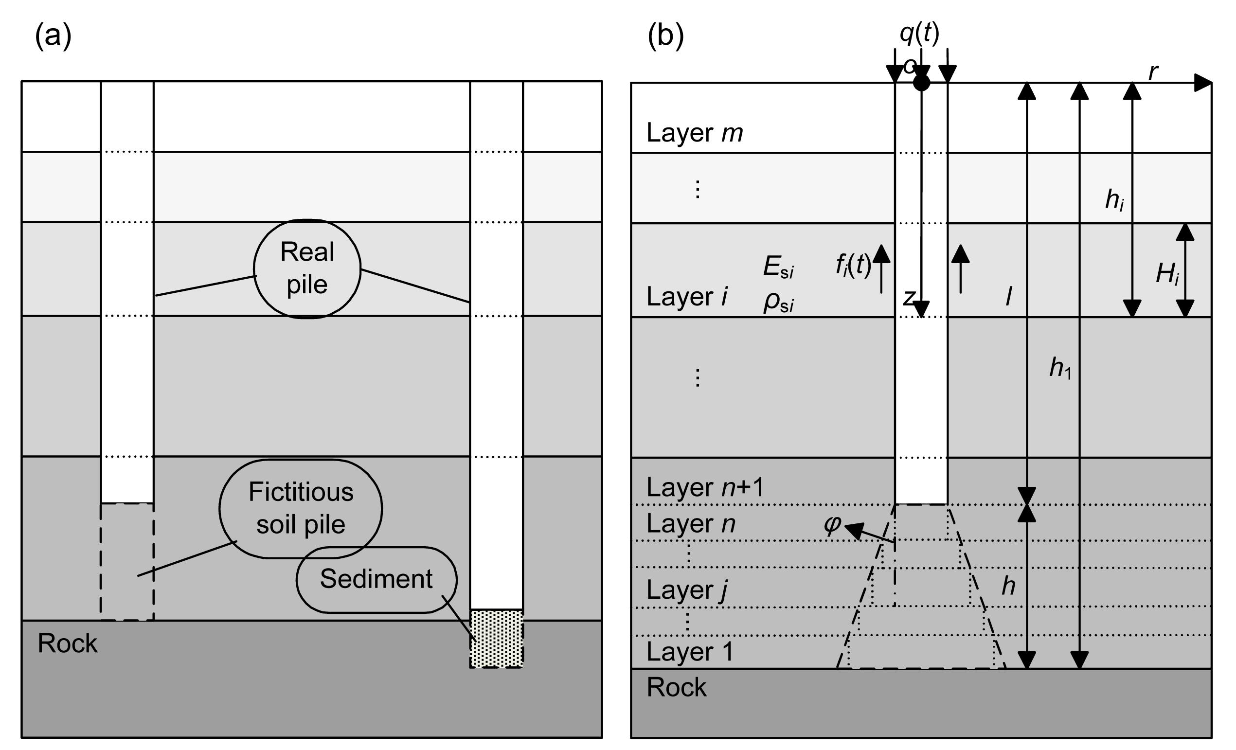
 According to the assumptions above, the pile was regarded to extend to the top of the bedrock; the soil column between the pile and the bedrock was treated as a virtual pile referred to as the fictitious soil pile in Fig. 1a. The fictitious soil pile has the same properties as the local soil and similar plane strain reaction as real piles. The displacement at the fictitious soil pile tip is restrained due to contacting with the bedrock. Novak and Beredugo (1972) and Novak (1977) presented some polynomial expressions for the dynamic parameters of the stiffness and damping at the pile tip and claimed that the expressions can be applied to different thicknesses between the tip and bedrock. Then, El Naggar and Novak (1994) proposed a similar method based on previous works of Novak (1972) and Novak et al. (1978). Nogami (1983) and Nogami and Konagai (1986; 1987) introduced a complete process of analyzing the linear or nonlinear dynamic response of piles or pile groups with a similar method in a time domain. However, the soil column model (CM) failed to consider the stress diffusion and thus underestimated the role of soil under the pile. Therefore, in this study, both the CM that is the same as Nogami (1983)’s (Fig. 1a) and the taper model (TM) that takes into account of the stress diffusion (Fig. 1b) were adopted as the fictitious soil pile model.




 In virtue of its simplicity, the CM can be applied to a number of problems, such as the analysis of piles with soft sediment at the pile tip (Fig. 1a).

 According to the continuum medium theory, the stress diffusion exists widely in the soil. When the stress diffusion with a diffusion angle φ is considered (Fig. 1b), it evolves to the TM model.

 Fig. 1b represents the soil-pile system. The soil in this model is divided into m layers, of which the first n layers are situated in the range of fictitious soil pile. Correspondingly, the pile is also divided into m elements. It should be noted that CM is a special case of TM in the particular situation when φ=0 or n=1.

3.  Assumptions

 The soil-pile system was developed based on the following assumptions:

1. The soil is a homogeneous, isotropic linear viscoelastic medium.

2. Only the vertical displacement of the soil is considered.

3. The pile is elastic and ideally vertical, treated as 1D bar with a uniform circular cross-section.

4. The stress and vertical displacement are continuous at the soil-pile interface, and the soil-pile system is subjected to small deformation harmonic vibration.

4.  Governing equations

 The plane strain model was adopted for the soil, in which only the vertical vibration was considered. The differential equation of equilibrium is (Novak et al., 1978) (1) , where ; is the dimensionless radius; r _0i is the radius of the ith element of pile, a _0i =ωr _0i /V _si is the dimensionless frequency; ω is the angular frequency of vibration; j is the imaginary unit; V _si is the shear wave velocity of the ith layer of soil; and, D _si is the material damping of the ith layer of soil.

 The initial and boundary conditions of the soil are assumed to be (2) , (3) .

 The solution of Eq. (1) can be expressed as (4) , where I₀() and K₀() are the first and the second kinds of zero order modified Bessel functions, respectively; and, A_i and B_i are constants determined by the boundary conditions.

 According to the boundary conditions of soil, B_i =0. Therefore, Eq. (4) is simplified as (5) .

 The vertical shear stress at any point in the soil is (6) , where ; G _si is the shear modulus of the ith layer of soil; and, K₁() is the second kind of the first order modified Bessel function.

 When r=r _0i , the complex shear stiffness of soil around the pile can be expressed as (7) .

 The axial response of the ith pile element is governed by (8) , where w_i is the axial displacement of the ith pile element; E _pi , ρ _pi , and A _pi are the Young’s modulus, density, and cross-section of the ith pile element, respectively; and, f_i =K_iw_i indicates the shaft friction of piles.

 The initial and boundary conditions of the pile can be expressed as (9) . At the pile head: (10) ; At the pile tip: (11) .

 Laplace transforms relevant to time is performed on Eq. (8) combined with the initial conditions: (12) , where .

 From Eq. (12), the following equation can be obtained: (13) , where , , V _si and V _pi are the shear wave velocity of the ith soil layer and the longitudinal wave velocity of the ith pile element, respectively; and ρ _si is the density of the ith soil layer; and, D _1i and D _2i are unknown constants determined by boundary conditions.

 Considering the boundary condition (Eq. (11)), Eq. (13) can be simplified as (14) .

 According to the definition of impedance, the complex impedance function at the top of the first pile element is expressed as (15) .

 Then, using the impedance transmission method, the complex impedance at the top of the ith element can be expressed as (16) , where , and k_i and c_i are the real stiffness and damping, respectively.

 When ξ=ωj, H _Vi (ω)=ωj/Z_i indicates the velocity response function in a frequency domain. Taking an inverse Fourier transform (IFT), the velocity response in time domain at top of the ith pile element subjected to unit impulse is obtained as follows: (17) .

 Therefore, the velocity response of pile undergoing arbitrary excitation of q(t) can be expressed as (18) , where .

5.  Numerical analysis

5.1.  Influence of fictitious soil pile element number

 As shown in Fig. 1b, the computation accuracy of complex impedance is significantly affected by the number of elements n. To determine the effect of n on the computation accuracy, three different values (n=10, 100, and 1000) are chosen for comparison. The soil is assumed to be homogeneous. The parameters of soil and pile are given in Table 1.




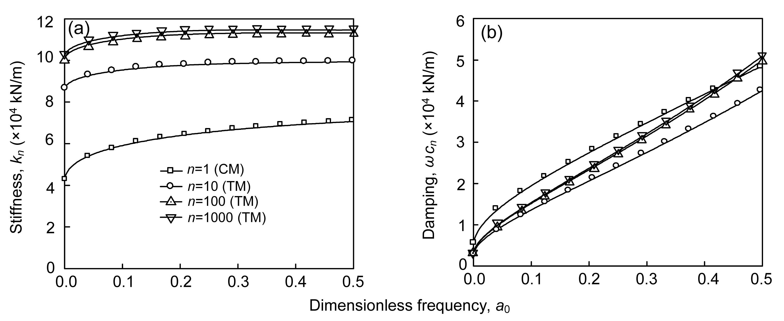
 In this section, the stiffness and damping at the pile tip for different values of n are presented. k_n is the dynamic stiffness at the pile tip; ωc_n represents the damping that reflects the dissipation of energy. The results of k_n and ωc_n for different n are shown in Fig. 2. It is noted that when n=1, the TM model will be reduced to the CM model. Theoretically, the number of n has no effect on the complex impedance in the CM model, so only the situation of the TM model is discussed. As can be seen from Fig. 2, when n=100 and 1000, the relevant complex impedances have no disparity, but when n=1 and 10, a smaller stiffness is obtained. It indicates that the TM model has a high astringency for the element number n. Therefore, in the following calculations, the value of n will be set to 100 to ensure calculation precision and improve computational efficiency.

5.2.  Influence of layer thickness between pile tip and bedrock on complex impedance of pile

 For the floating pile, Novak (1972; 1977) put forward a method to simulate the stiffness and damping at the pile tip in a frequency domain and suggested some polynomial expressions under specific conditions. In this segment, one of Novak (1977)’s suggestions was adopted and was then compared with the current method of fictitious soil pile. When Poisson’s ratio of soil is 0.25, the polynomial expressions suggested by Novak (1977) for the parameters of complex impedance are (19)

 The stiffness and damping at the pile tip can be expressed as (20) , where G _s is the shear modulus of the soil below the pile tip, and r ₀ is the radius of pile.

 Novak (1977) deemed that if the layer thickness between the pile tip and the bedrock h is less than about 5r ₀, Eq. (19) would be inappropriate to be applied due to the increase of C _w1 and the decrease of C _w2. In Figs. 3 and 4, the CM and TM models were adopted to analyze the influence of h on the complex impedances at the tip, respectively, and their results were compared with Novak (1977)’s solution. The main properties of soil and pile used in calculation are listed in Table 1.

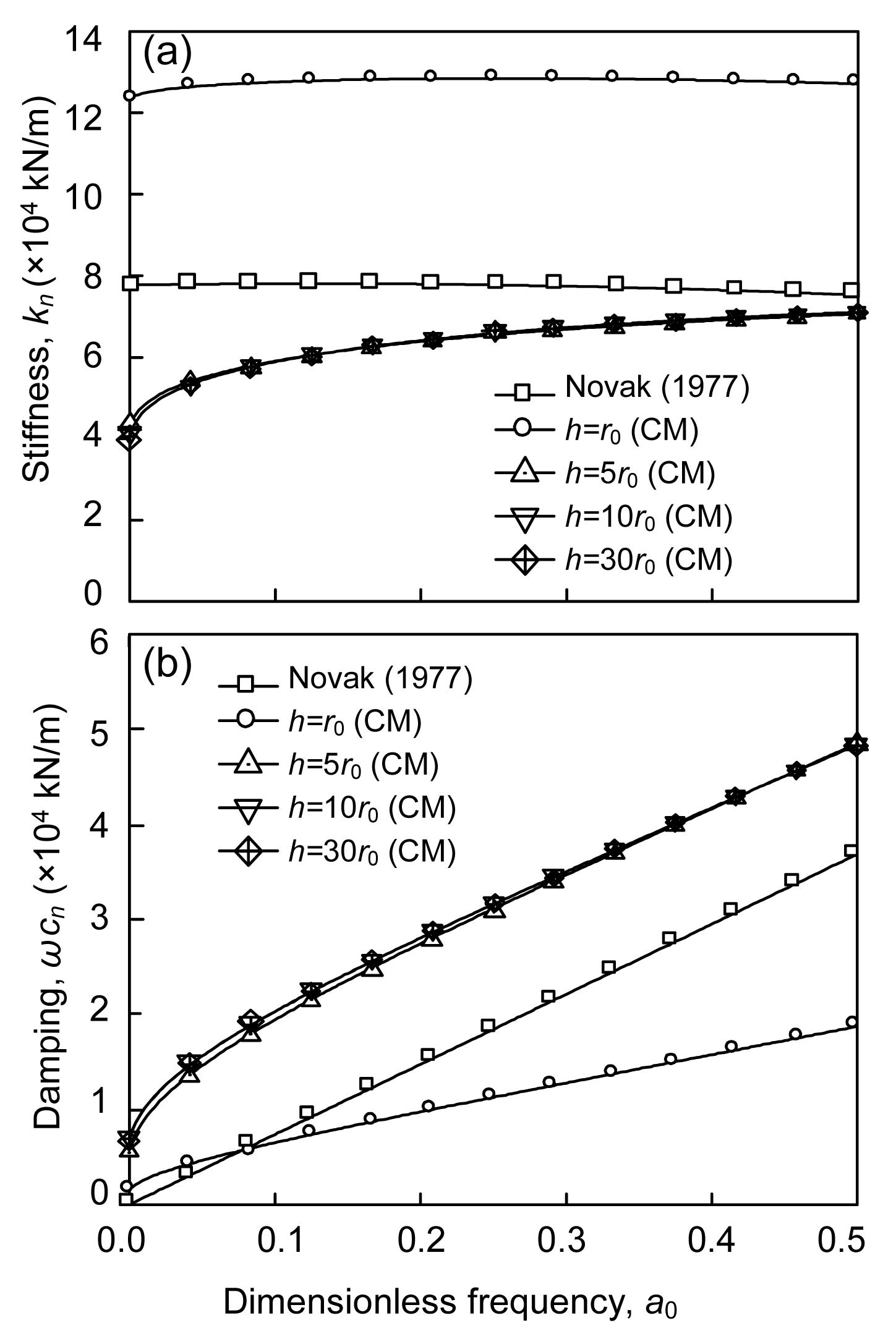
 Fig. 3 shows the stiffness and damping at the pile tip for various values of h based on the CM model. It is observed that when h=r ₀, the impedance has a great difference compared with other results using larger values of h. It is also noted that the stiffness k_n is larger while the damping ωc_n is smaller, which coincides well with Novak (1977)’s conclusion. When h=5r ₀, 10r ₀, and 30r ₀, the three curves of impedance are overlapped. That is, the impedance will maintain at a relatively stable level when the thickness of the stratum under the pile comes to a certain value, 5r ₀, for instance. The value of the stiffness suggested by Novak (1977) is larger than those obtained by the CM model for a certain a ₀ when h≥5r ₀, but the damping shows an opposite tendency.




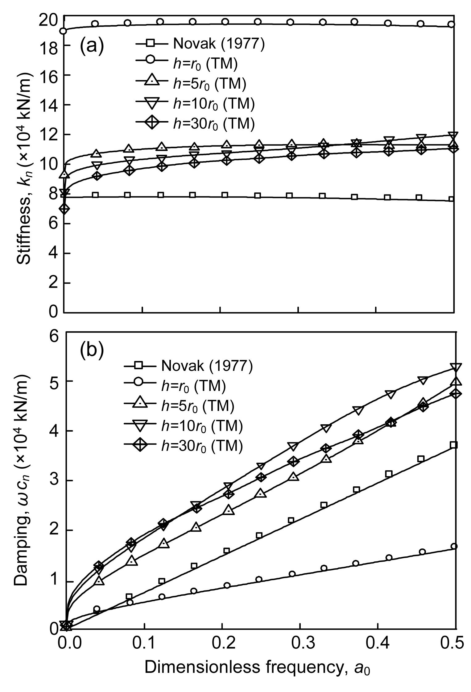
 Unlike the CM model, there is an obvious difference in complex impedances when h≥5r ₀ in the TM model. All the stiffness and damping values are larger than those presented by Novak (1977). Generally when h exceeds 5r ₀, the complex impedance at the pile tip will remain at the same level, in line with the conclusion of Novak (1977), except for a little discrepancy between the curves shown in Fig. 4.




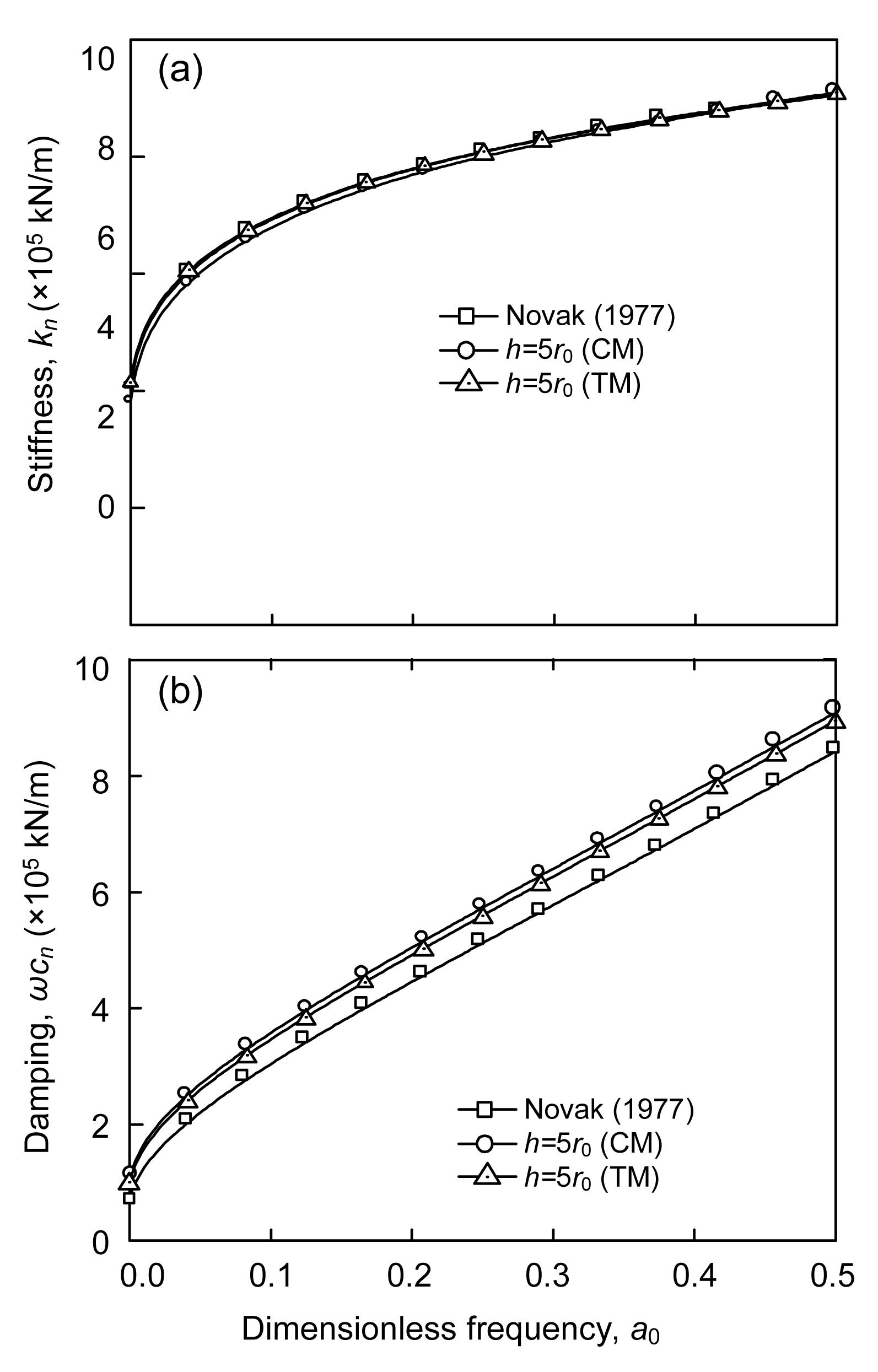
 From the above analysis, it can be seen that the complex impedance at the pile tip solved by the fictitious soil pile model is in good agreement with Novak (1977)’s suggestion. To further verify the validity of fictitious soil pile model, the impedances at the pile head were discussed in Figs. 5 and 6, respectively, for floating piles and end bearing piles.

 In Fig. 5, three cases were investigated for the complex impedance at the pile head. The stiffness curves illustrate that the present method is as reasonable to analyze the dynamic problem of floating pile as Novak (1977)’s method, especially the TM model. Meanwhile, the damping curves are almost with the same slope, which demonstrates the validity of the current models.




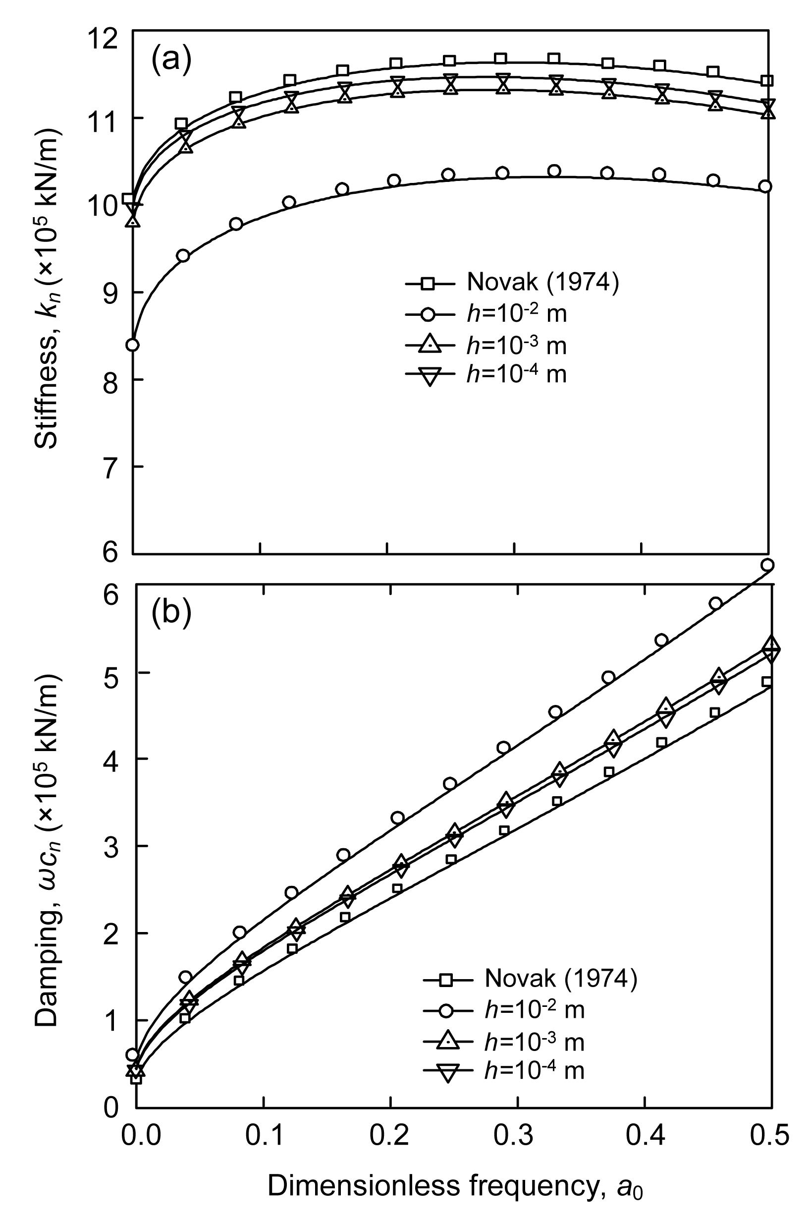
 For the end bearing pile, a very small value of h can be adopted to model the condition at the pile tip. In Fig. 6, h=10⁻², 10⁻³, and 10⁻⁴ m were taken into consideration, and the results were compared with the solution presented by Novak (1974). It is obvious that the impedances at the pile head in the present study are close to the solution of Novak (1974) with the decrease of h, which means that the fictitious soil pile model can also be used to solve the vibration problem of end bearing piles embedded in soil.

5.3.  Influence of layering property of soil under pile tip on complex impedance of pile

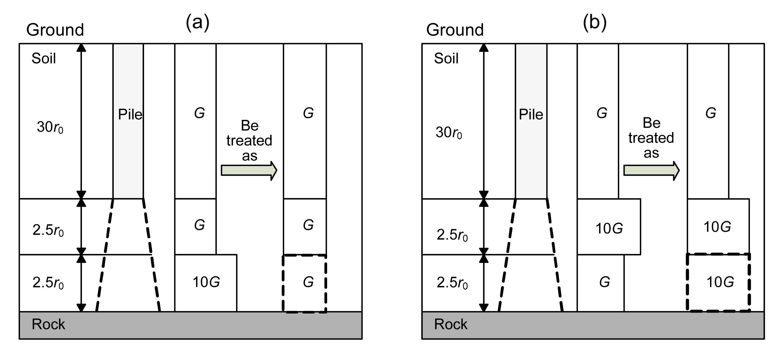
 The layering of stratum beneath the pile tip, which was neglected in the model presented by Novak (1977), is taken into consideration in the current approach. Two cases were discussed in Fig. 7. Here, the density and Poisson’s ratio of soil and pile given in Table 1 were also adopted. Furthermore, r ₀=0.25 m and G=58.32 MPa. 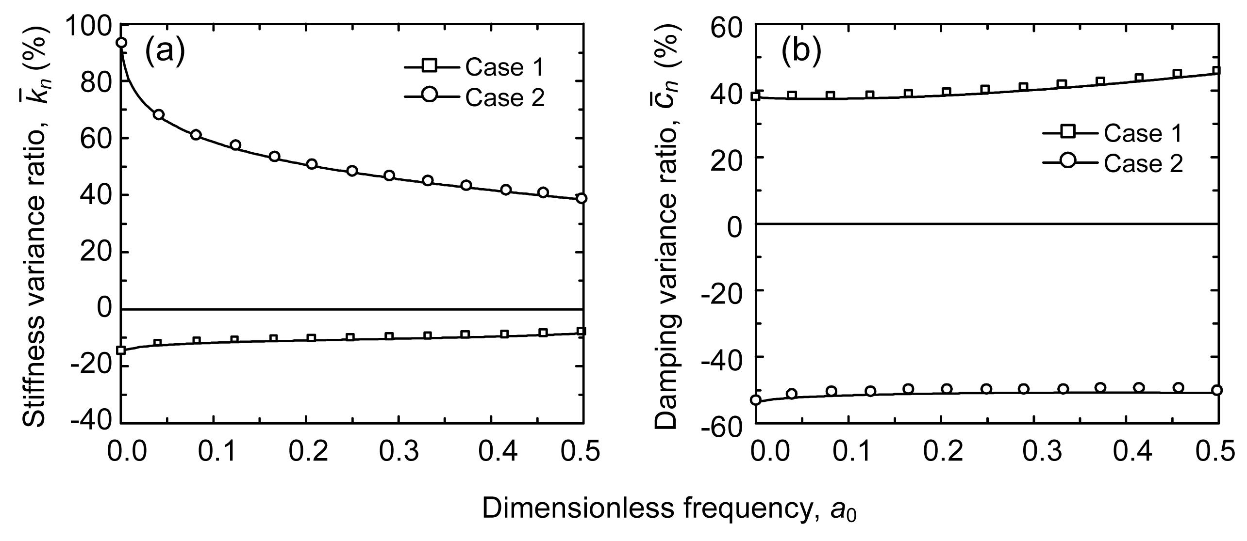To identify the effect of soil layering, two dimensionless values of stiffness and damping are defined as (21) where the subscript ‘L’ indicates the consideration of the layering of soil. Fig. 8 represents the errors of complex impedance at pile tip due to neglecting the soil layering in two cases. As shown in Fig. 8, the stiffness is 10% smaller and the damping is 40% larger than the values with consideration of the soil layering in Case 1. In Case 2, the errors are more significant and have exceeded 40% for both stiffness and damping, which is less conservative.

6.  Applications of fictitious soil pile model

6.1.  Application I

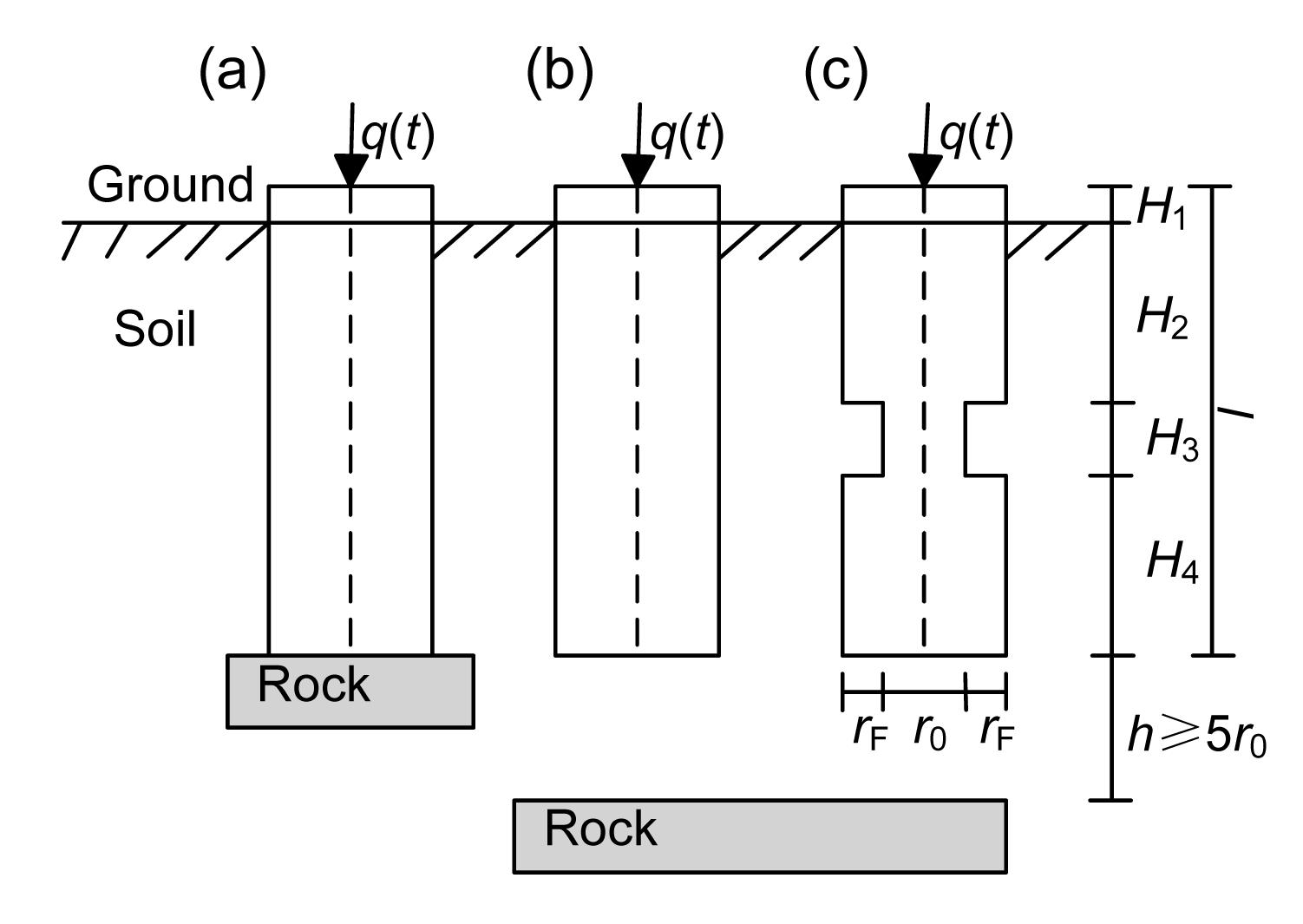
 In this section, the TM model was used to study the velocity response at the top of intact and defective piles under impulse load. Liao and Roesset (1997a; 1997b) reported a case of testing the integrity of the pile shaft. In this study, Liao and Roesset (1997a; 1997b)’s case was collected for discussion with the current approach. The dimensions of three kinds of piles are shown in Fig. 9. l and A _p are the length and the cross-sectional area of the piles respectively, l=12 m and A _p=0.785 m²; H_i (i=1, 2, 3, 4) indicates the length of ith part of pile; and r _F is the width of defect. The properties of piles and soil are listed in Table 2.







 Assuming the pile is subjected to a semi- sinusoidal excitation force as follows: (22)

 Substituting Eq. (22) into Eq. (18), the velocity response function in time domain can be expressed as (23) , where m represents the pile head.

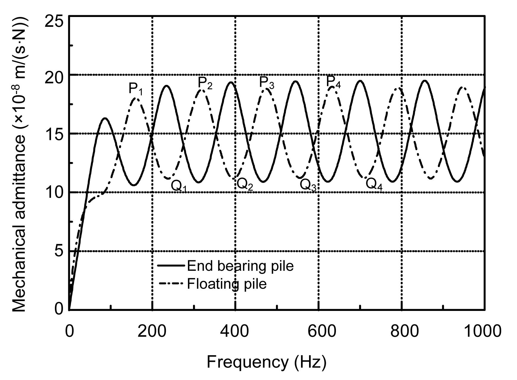
 The mechanical admittance method (Fig. 10) and the impulse response method (Fig. 11) are applied to analyze the velocity response at the pile head. Fig. 10 shows the velocity admittances of intact piles in frequency domain. According to Davis and Dunn (1974), the length and the cross-sectional area of the pile can be approximately computed by (24) , (25) , where V _p is the longitudinal wave velocity in the pile; ∆f is the frequency interval between two similar peaks (or troughs) of the response curve in the steady-state region; ; and, ρ _p is the density of pile.







 In Fig. 10, the phase separation between the two curves is about half a period, which represents different reflected signals at the pile tip in Fig. 11. All the peaks are very similar for intact piles in the steady-state region, so the frequency interval between two arbitrary consecutive peaks, referred to as ∆f, can be used to estimate the length and cross-sectional area of the pile by Eqs. (24) and (25).

 For floating piles:

  ,

  ,

  ,

  ,

  ,

  .

 For end bearing piles:

  ,

  ,

  ,

  ,

  ,

  .

 The results are summarized in Table 3. It is observed that the error between the theoretical length and actual length of the pile is very small. Compared with the results of Liao and Roesset (1997a; 1997b), the current approach is more accurate in estimating the cross-sectional area of the pile.




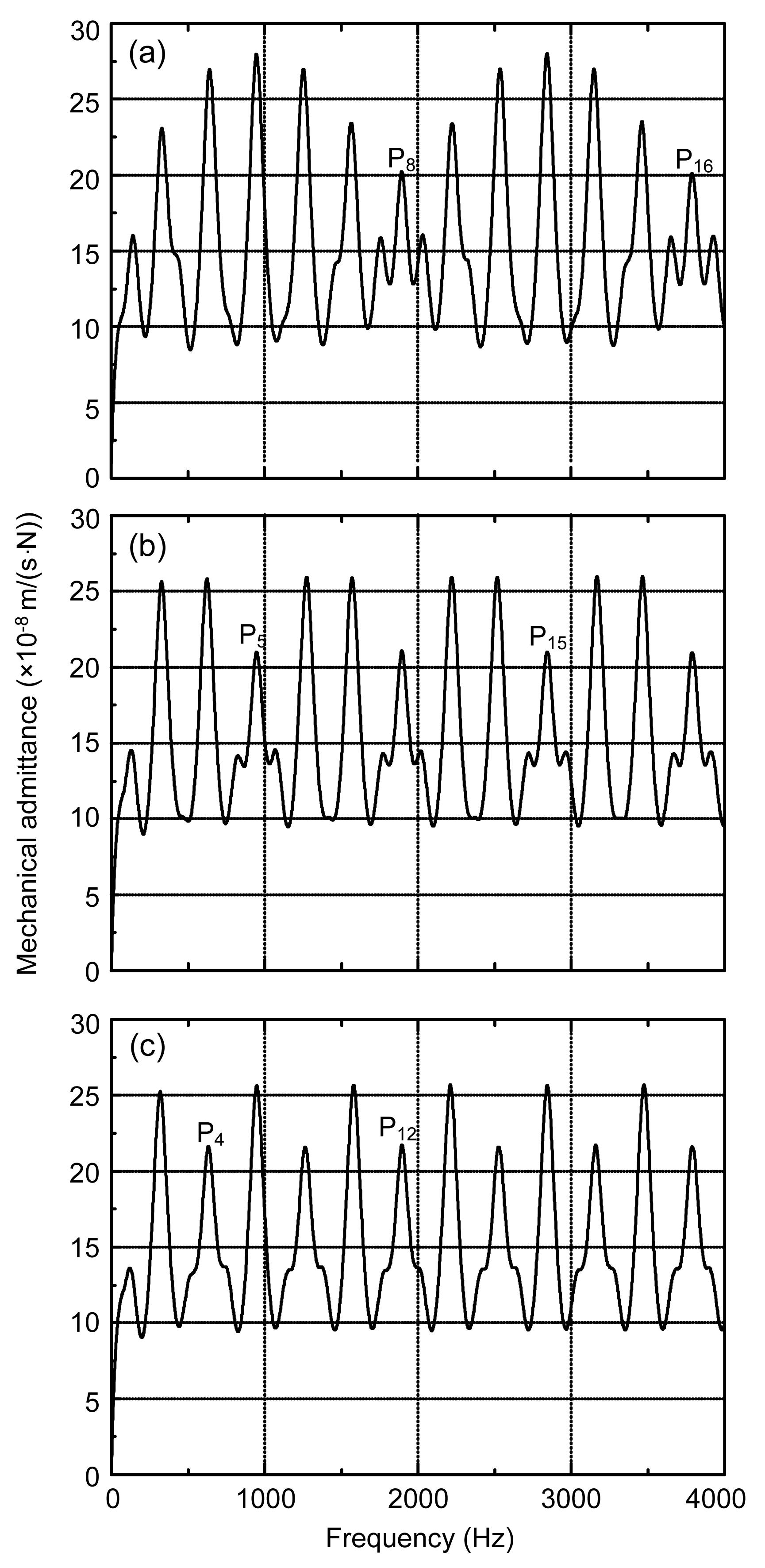
 The pile with a neck shown in Fig. 9c was studied as the length of the neck, H ₃, increased from 1 to 3 m. The mechanical admittance and impulse response are shown in Figs. 12 and 13, respectively. The determined results of the length of the neck are listed in Table 4.




 As shown in Fig. 12, the peaks used to calculate the neck length have distinctive features, which are larger than the adjacent peaks. This phenomenon is in a good agreement with the study of Liao and Roesset (1997b). The estimations about the length of the neck shown in Table 4 demonstrate that the current approach is stable to identify the defects in piles.




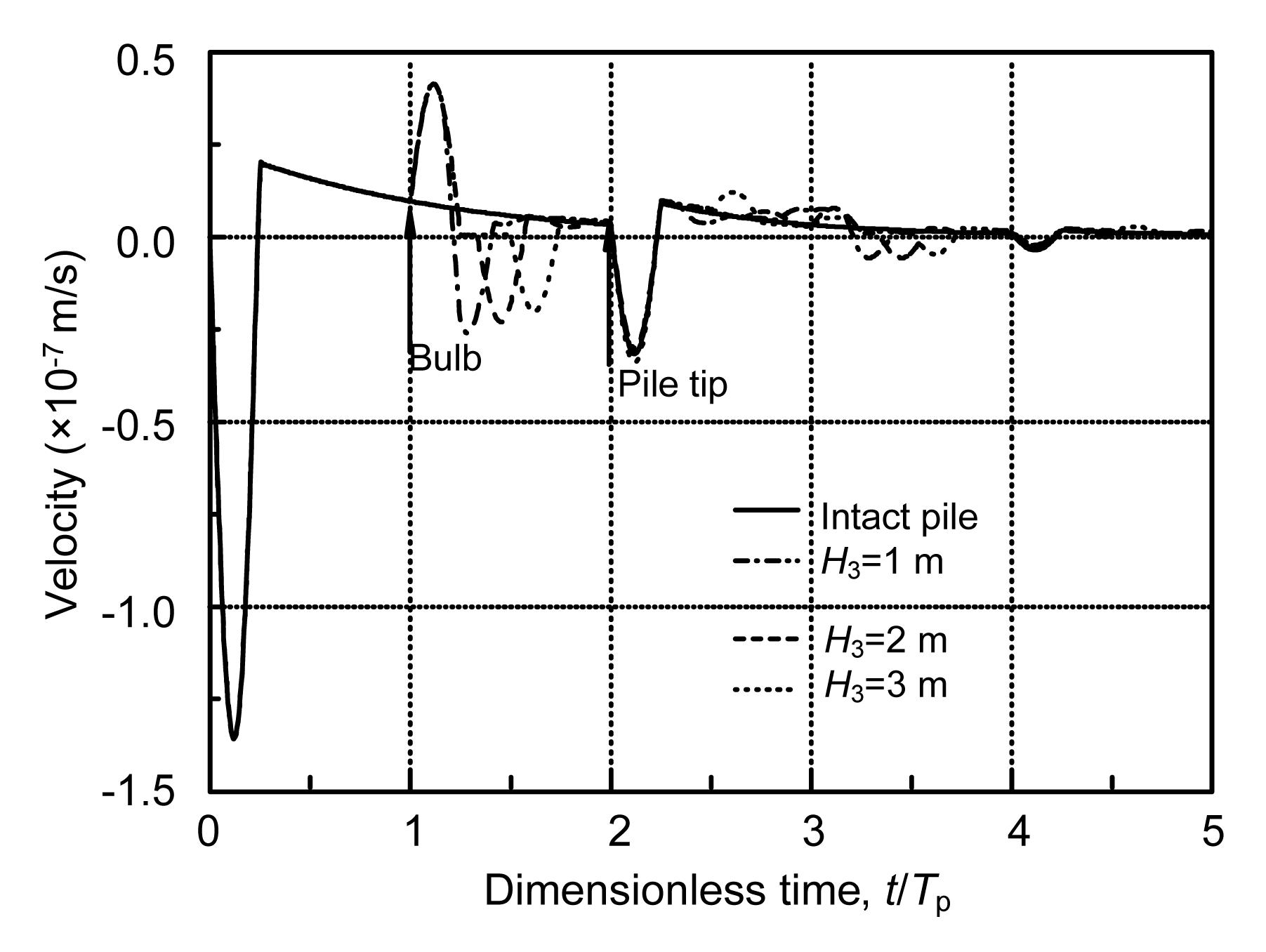
 In Fig. 13, T _p=l/V _p, consequently, if t/T _p=2, the relevant velocity represents the reflected signal at the pile tip. When t/T _p=1, the reflected signals resulted from the relevant defect can be clearly observed. Compared with Case I, it is easy to identify the length of the defect in Cases II and III. Thus, for the pile with a short defect, a combination of the mechanical admittance method and impulse response method is a good choice for the calculation of the length of defect. From Fig. 13, it is also observed that the reflected signal at the pile tip is diminished due to the neck length.

6.2.  Application II

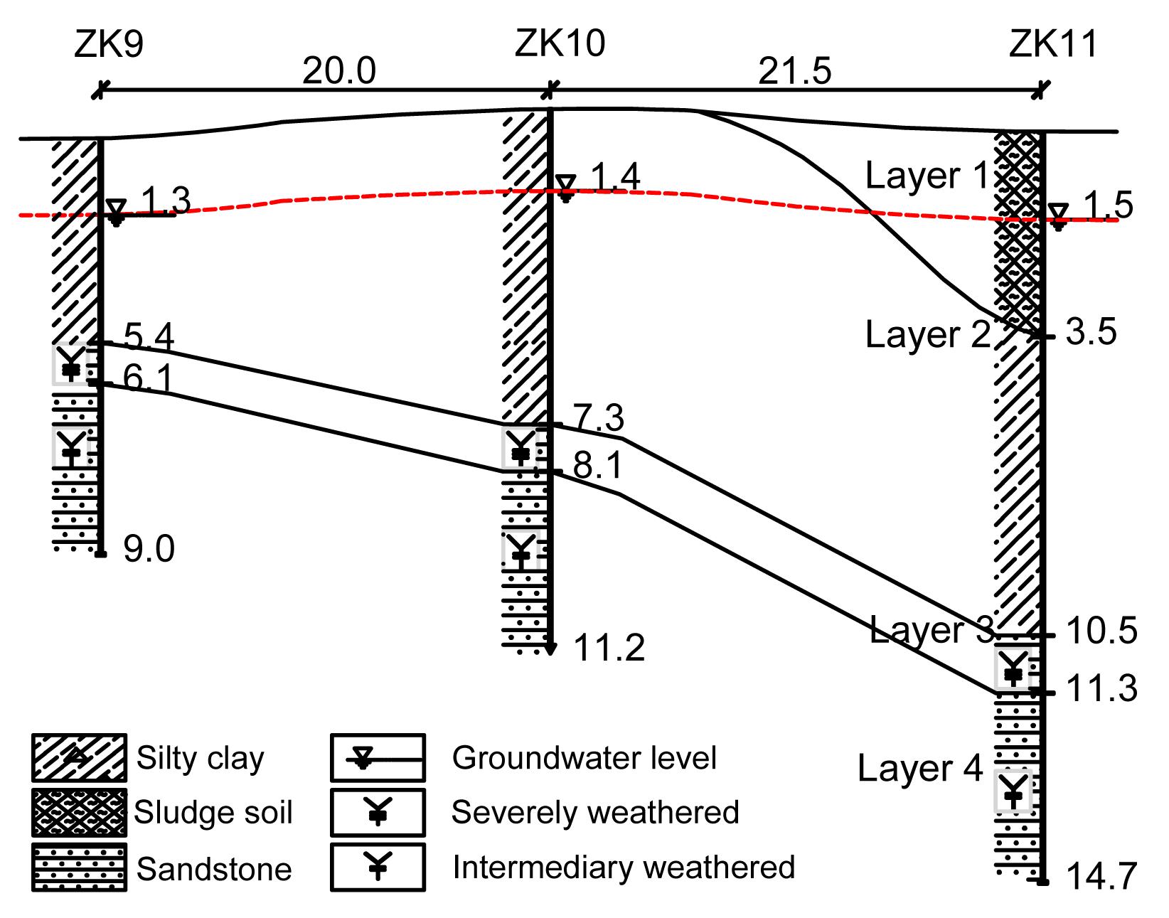
 The behavior of the pile with sediment under the pile tip was analyzed based on the CM model. The project site is located near the Qiantang River in the city of Hangzhou, China. Fig. 14 depicts the typical soil profile, and Table 5 lists the soil parameters of this project. In this project, bored piles were applied, and the ground layer of intermediary weathered sandstone was selected as the bearing stratum. The investigated piles are located near the borehole of ZK11. The radius of the piles is 0.4 m; the length of piles is 10.3 m, with a depth of 1.2 m embedded in the bearing stratum. The thickness of sediment, h, is limited to 5 cm. The mass density and longitudinal wave velocity of piles are 2400 kg/m³ and 3800 m/s, respectively.







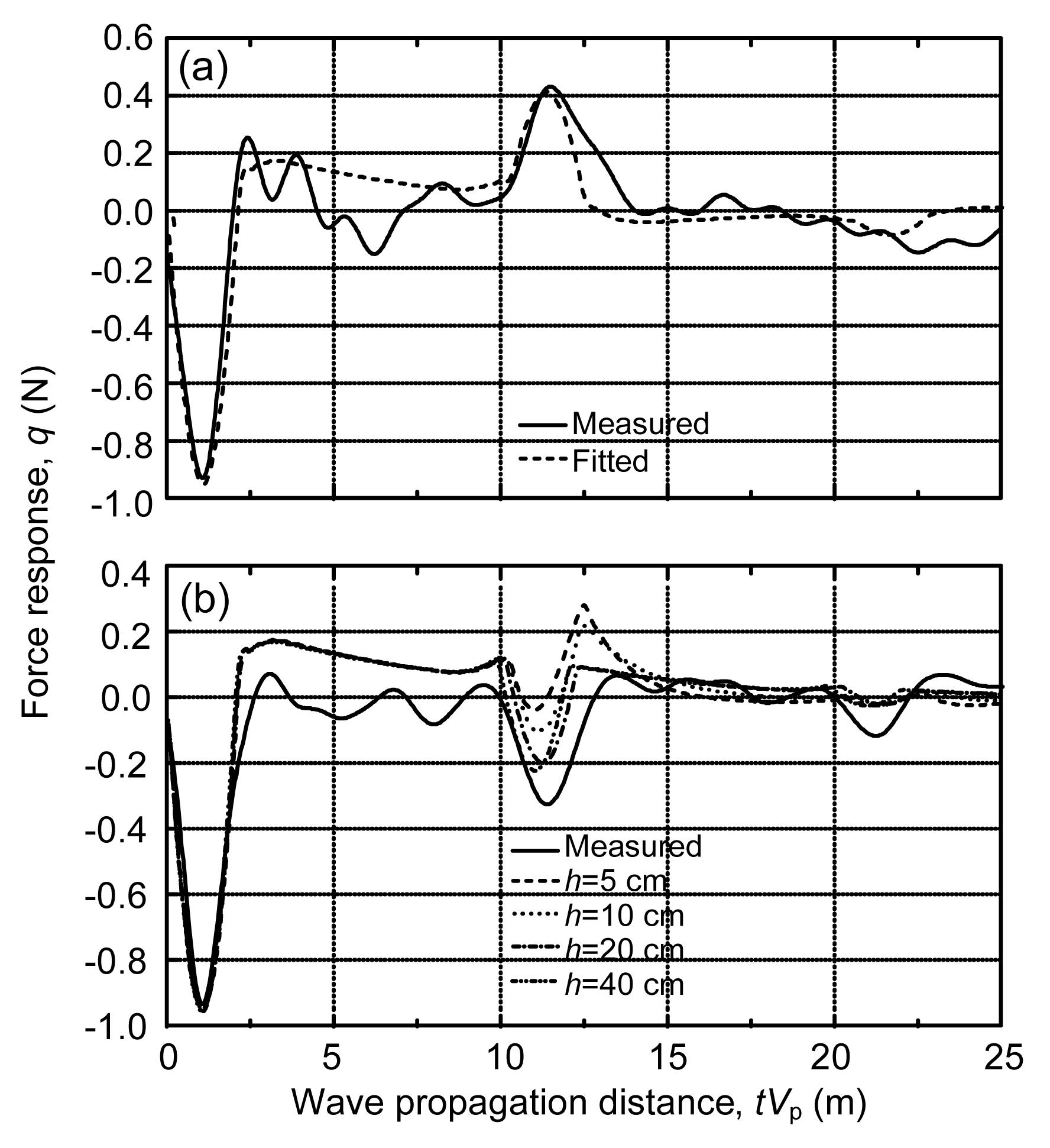
 In Fig. 15, two integral detecting charts of engineering piles are illustrated. The longitudinal coordinate q represents the force response at the pile head, which is equal to V/(V _p ρ _p A _p), where V is the velocity response. According to the shape of the reflected signal of q, the horizontal axis tV _p can be used to determine the length of the pile.




 From the curve of the detected signal at the pile head in Fig. 15a, it can be inferred from the signal of the response reflected at the pile tip that the investigated pile is rested on a rigid layer. Based on this assumption, let the thickness of the sediment approach zero, i.e., h→0 m, the fitted results were obtained using the fictitious soil pile model. It is found that the fitted results are in a good agreement with the measured response.

 In Fig. 15b, the detected signal at tV _P≈10 m in the measured curve suggests that the soil under the pile tip is weak based on the theory of low strain integrity testing. However, since the two piles under investigation are very close to each other, the possibility of weak underlying stratum is excluded. Hence, it is deduced that there is sediment under the pile. From the four fitted curves with different thicknesses of sediment h, it can be observed that the fitted curve of h=20 cm is the closest to the actual signal, which implies that the thickness of the sediment is about 20 cm. From the fitted curves, it is shown that the adopted model can provide a good prediction of the thickness of sediment.

 The above cases demonstrate that the fictitious soil pile method can give sufficiently accurate results in detecting the existence of sediment under the pile tip. As for the influence of the sediment thickness on the complex impedance at pile head, a quantitative analysis will be presented as below, where the parameters in Table 5 were adopted.

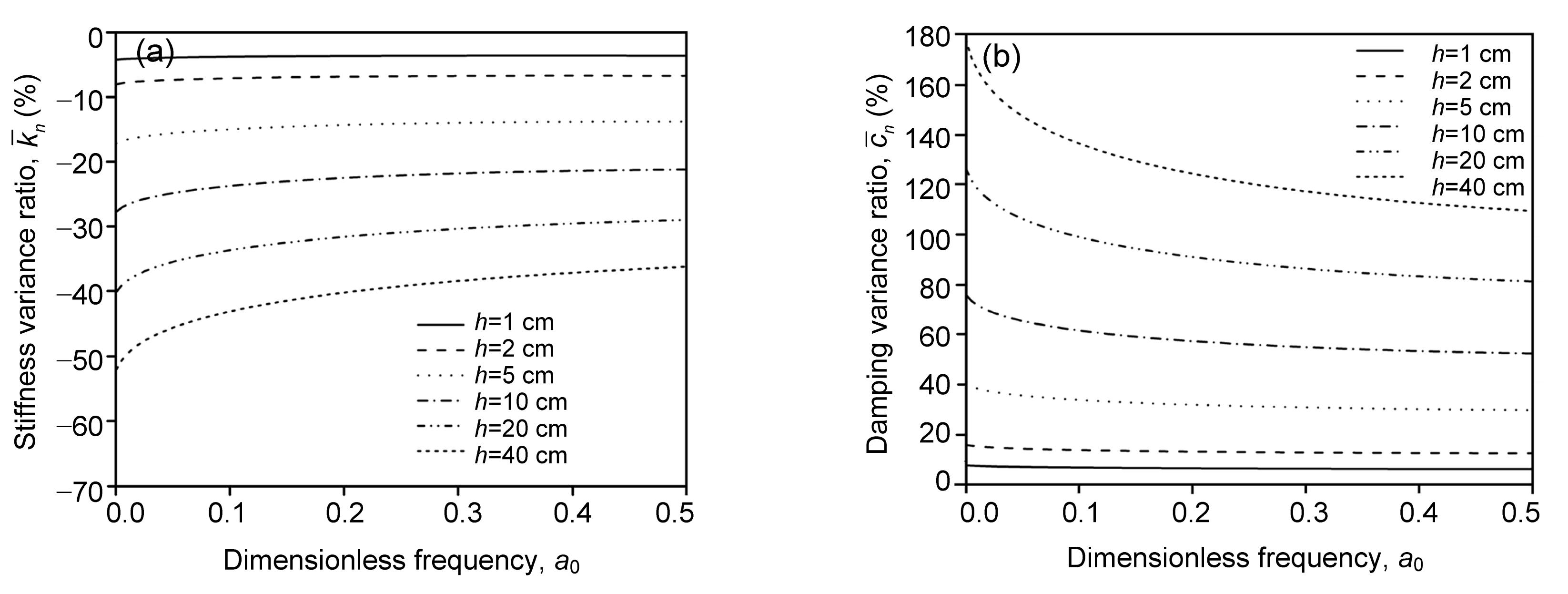
 Eq. (21) was adopted to calculate the effect of sediment on the complex impedance at the pile head. Here, k _L and c _L were replaced by k _B and c _B, respectively, where the subscript ‘B’ represents end bearing pile, so k _B and c _B are the stiffness and damping of a good end bearing pile, respectively. k and c represent the stiffness and damping with different values of h, respectively. Positive values of and represent increases, and negative values for decreases.

 Fig. 16 shows the results of and in a frequency domain under six different values of h. All the values of are negative. When h=1–2 cm, =−5%–−8%; h=5 and 10 cm, reaches −15% and −22%, respectively. When the thickness of sediment is 20 cm, the stiffness will decrease about 30%. For a lower frequency, the influence of sediment on stiffness is more apparent. For example, when h=20 cm and a ₀→0, =−40%. Therefore, for the piles undergoing a long-term static load, the control of sediment should be paid more attention.




 The positive values of reflect that the sediment can lead to the increase of damping. The change of damping caused by the sediment is greater than that of stiffness. For instance, the increase of damping will exceed 30% for h=5 cm, and 80% for h=20 cm.

 Generally, when the thickness of the sediment layer is relatively large, the stiffness at the pile head is lower and the damping is higher.

7.  Conclusions

 A named fictitious soil pile model for analyzing soil-pile interaction problems at the pile tip was constructed in two different forms, which are referred to as the CM and TM, respectively. Furthermore, an analytical solution was proposed to compute the complex impedance at the pile head and tip. By discussing the complex impedance and velocity response of piles, conclusions were drawn as follows.

1. Comparison results between the current method and Novak (1977)’s study demonstrated that the current method is in good accordance with Novak (1977)’s. For floating piles, the complex impedances at the pile tip suggested by Novak (1977) are between those in the CM and TM. When the depth of soil under pile tip h exceeds about 5r ₀, the influence of the soil on the stiffness and damping at the pile tip will remain at the same level. For end bearing piles, the current method is also applicable by assuming h→0. Therefore, our method avoids using different equations and boundary conditions to analyze different piles.

2. Stress diffusion is not incorporated in the CM model (Nogami, 1983), which is over conservative and restricted to the specific conditions. By contrast, TM model is more appropriate and realistic for the consideration of the real stress state of the soil. Compared with the method proposed by Novak (1977), which needs to reselect the formula with the changing of the soil state, the current approach is more convenient in calculating the stiffness at the pile tip.

3. Two cases for multilayer stratum under the pile tip were studied and the influence of the soil layering, was identified in this paper. In this case study, about 10%–40% errors of the complex impedance are generated due to the neglect of the soil layering.

4. Two applications of the current approach were given. In the first application, the mechanical admittance method and impulse response method were used to analyze the velocity response of intact and defective piles by the TM. It was found that the TM could identify the defects in piles with a satisfactory precision. Furthermore, the admittance phases between floating pile and end bearing pile have a distance of about half a period, which points to different reflected signals in impulse response method. For the pile with a short defect, a combination of mechanical admittance method and impulse response method has been proven to be a good choice to determine the length and position of defects. In the second application, the pile sediment left in a drilling process was analyzed based on the CM. The results of analysis implicated that the sediment could lead to the decrease of stiffness and increase of damping, especially for the pile subjected to low frequency loads. The numerical values demonstrated that the stiffness at the pile head will decrease about 15% when the thickness of sediment was 5 cm. Therefore, it is emphasized that the sediment should be restricted in practice.

 From the above, it could be concluded that the new model established in this paper satisfactorily simulates the interaction between the soil and the pile tip, which provides a new insight into the soil-pile coupling problem at the pile tip.

---

* Project (No. 50879077) supported by the National Natural Science Foundation of China