Similar articles

Abstract: Recently, the finite element method (FEM) has been commonly applied in the engineering analysis of rotor dynamics. Gyroscopic moments, rotary inertia, transverse shear deformation and gravity can be included in computational models of rotor-bearing systems. In this paper, a finite element model and its solution method are presented for the calculation of the dynamics of dual rotor systems. A typical structure with two rotor shafts is discussed and the procedure for obtaining the coupling motion equations of the subsystems is illustrated. A computer program is developed to solve critical speeds and to simulate the transient motion. The influence of gyroscopic moments on co-rotation and counter-rotation is analyzed, and the effect of the speed ratio on critical speed is studied. The dynamic characteristics under different conditions of increasing speed during start-up are demonstrated by comparison with transient nodal displacements. The presented model provides a complete foundation for further investigation of the dynamics of dual rotor systems.

1.  Introduction

 Despite the extensive use of the transfer matrix method in rotor dynamics problems, the finite element technique has become more popular recently for its high efficiency and convenience of modeling. The finite element method (FEM) for rotors was first developed by Ruhl and Booker (1970). Nelson and Mc-Vaugh (1976) extended it to include translational and rotary inertias, gyroscopic moments, and axial loads, and Nelson (1980) considered the effect of shear deformation using the Timoshenko beam theory. With the application of this method, we are able to solve complex problems because the equations of motion are explicit and easier to couple with bearing flexibilities or other multiple excitations.

 Dual rotor systems are widely used in aircraft engines because they can reduce the influence of gyroscopic moments generated by high and low pressure rotors when counter-rotating. Research on the dynamic characteristics of dual rotor structures is of great significance for lowering vibration and noise, and can enhance their overall performance, including their reliability and stability. In a dual rotor system, because of the inclusion of a special inter-bearing which connects the inter rotor with the outer rotor, the corresponding force becomes more complicated. The equations of the two subsystems should be coupled. This is the key difference between a dual and a single rotor system in terms of mathematical modeling. Critical speed prediction of a typical dual rotor system was first proposed by Rajan et al. (1986). Hsiao-Wei et al. (2002) carried out a systematic theoretical analysis and an analysis of the effects of the speed ratio and inter-bearing stiffness. However, little attention has been focused on the transient motion, which is becoming increasingly important in understanding the dynamic behavior when a rotor starts up, stops, or goes through a critical speed.

 In this paper, based on the studies of Nelson (1976) and Hsiao-Wei et al. (2002), a computational model of a dual rotor bearing system is established under an inertia coordinate. The procedure integrates the advantages of FEM and the Newmark method (1959) to obtain natural frequencies, critical speed maps, and transient results. The basic process for extending this model to a more complex rotor-bearing system such as a triple rotor system and geared rotors is also presented.

2.  Component equations

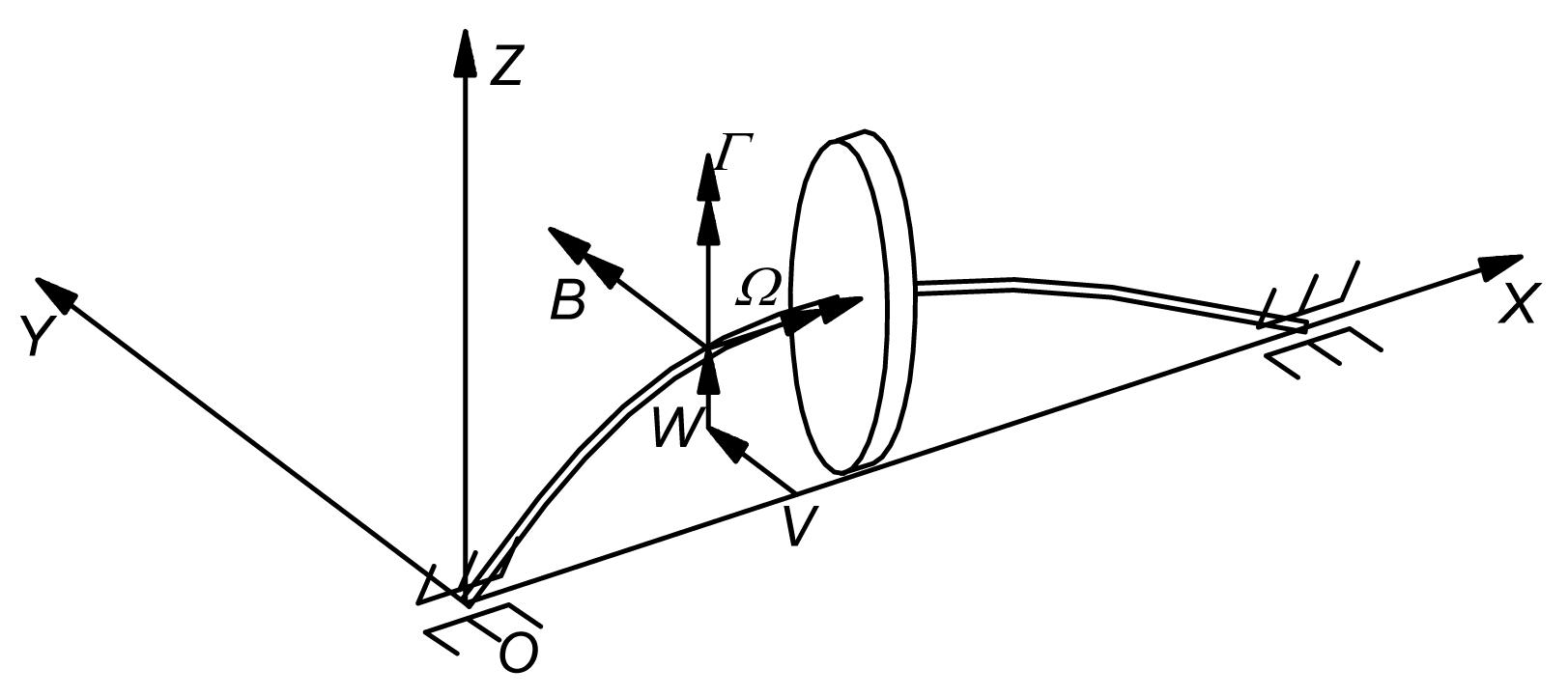
 A typical flexible rotor-bearing system with a single rotating shaft consists of a rotor, rotor segments and discrete bearings (Fig. 1) along with an inertia coordinate frame. The rotor is composed of discrete disks and the rotor segments have distributed mass and elasticity.




 Expressions of kinetic energy and strain energy are necessary to characterize the disk and shaft element. Lagrange’s formulation is applied to obtain the differential equations of motion for each component. The formulation is written in the form (1) , where T and U are the kinetic and strain energies, respectively, u_i are generalized independent coordinates and Q_i are generalized forces.

2.1.  Angular velocity and coordinates

  OXYZ is an inertia coordinate, in which O is coincident with the center of the rigid disk and the X axis is collinear with the undeformed rotor center line. OX ₃ Y ₃ Z ₃ is attached to the disk and rotates synchronously with the rotor. The relationship between them can be described by the following successive rotations: OXYZ rotates θ_z about OZ, yields OX ₁ Y ₁ Z ₁; OX ₁ Y ₁ Z ₁ rotates θ_{y 1} about OY ₁, yields OX ₂ Y ₂ Z ₂; and OX ₂ Y ₂ Z ₂ rotates θ_{x 2} about OX ₂, yields OX ₃ Y ₃ Z ₃, where , , and ; &phgr; is the angle of rotation about X and Ω is the spin speed, and the angular velocity of OX ₃ Y ₃ Z ₃ is (2) , where , and are rotation matrices.

2.2.  Rigid disk

 For a typical rotor disk, strain energy is neglected in view of the rigid body assumption, and it can be modeled as a four-degrees-of-freedom element. The vector of generalized coordinates includes the displacements V, W and the corresponding slopes B, Γ. With the application of the angular velocity of OX ₃ Y ₃ Z ₃, the kinetic energy of the disk for lateral motion is given by (3) , where m _D is the disk mass, J _d denotes the diametral inertia and J _p denotes the polar inertia. 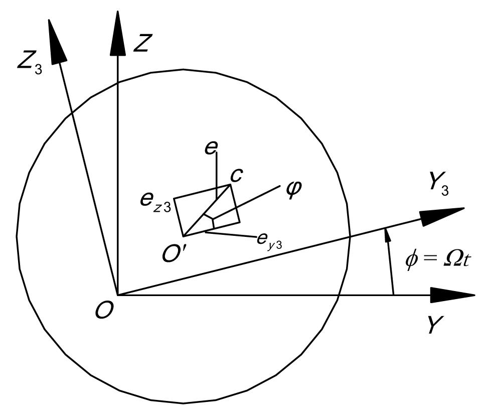Following the Lagrangian approach, we can obtain: (4) , where M _D is the mass matrix of the disk element and its gyroscopic matrix is G _D. The unbalance force (Fig. 2) caused by the eccentric mass is (Carrella, 2009) (5) , where e is the eccentricity, φ is the phase of unbalance, and the disk mass center is located at (e _y3,e _z3) in OX ₃ Y ₃ Z ₃. When gravity needs to be considered, the item is included (Appendix).

2.3.  Finite shaft element

 Fig. 3 shows a two-node shaft element with eight degrees of freedom. The time displacements of an arbitrary cross section in the element can be expressed by the product of its nodal displacements and shape functions (Michael et al., 2010).




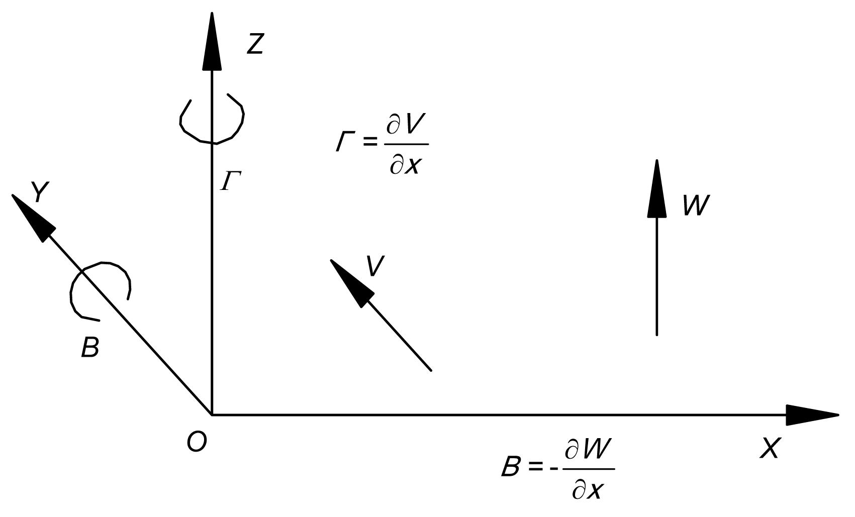
 According to the geometric analysis in Fig. 4, the slopes (B, Γ) can be given by the following relationships (Jei and Lee, 1988): (6) , (7) .




 For the shaft element the vector represents the generalized coordinates. The interpolation functions (N ₁, N ₂, N ₃, and N ₄) are used to calculate the nodal displacements, and the expressions are given by (8) , (9) , (10) , (11) .

 The corresponding velocities are calculated by taking derivatives with respect to time. Similarly, the kinetic energy is obtained by computing an integral over the length of the element (Rao et al., 1998): (12) where μ, j _d and j _p are the shaft element mass, diametral inertia and polar inertia per unit length, respectively.

 For a differential element with a thickness of ds and located at s, the potential energy of elastic bending is (Rao, 1996) (13) , where E is the Young’s modulus, and I is the second moment of area.

 Integrating the and following the Lagrangian approach, we can obtain: (14) , where , , and are the translational mass, rotatory mass, gyroscopic and stiffness matrices of the shaft element, respectively.

 Based on the principle of virtual displacement, the gravity force vector can be deduced (Appendix). The virtual work of the gravity effect is (15) .

2.4.  Bearing

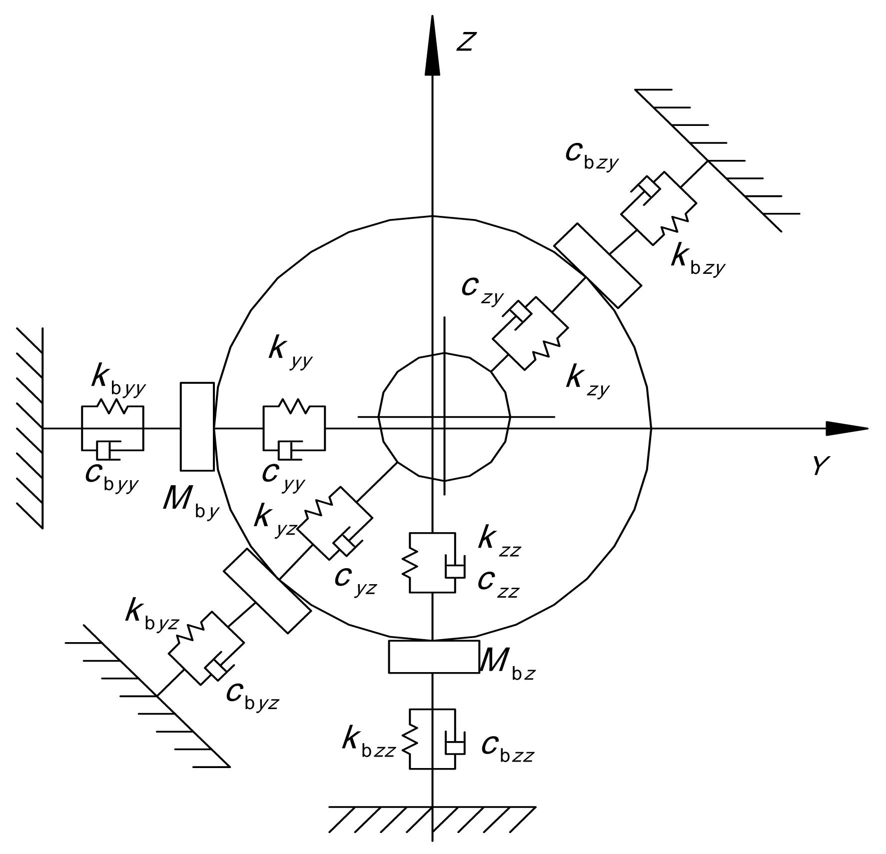
 With the assumption of little vibration, the inherent nonlinear characteristics of fluid-film bearings can be linearized at the static equilibrium position (Zhong, 1987; Abduljabbar et al., 1996). Then its governing equation can be expressed as (16) , where are the displacements of the bearing node and are the displacements of the journal node. M _b, C _b1, K _b1, C _b2 and K _b2 are included (Appendix), and the elements of the matrices are illustrated in Fig. 5. The generalized force acting on the journal is (Das et al., 2008) (17) .




 In the case of a high stiffness foundation, V _b=W _b=0, and the equation is simplified to (18) .

3.  Assembly and system equations

3.1.  System of a single rotating shaft

 Fig. 6 shows a rotor-bearing system with a single rotating shaft. The vibration equation of the rotor can be obtained by combining Eqs. (4) and (14) (Shiau et al., 1999): (19) , Fig. 6

Typical rotor-bearing system

where M ^s, G ^s and K ^s are the mass, gyroscopic and stiffness matrices, respectively of the rotor system, and u ^s is the vector of its generalized coordinates. is the unbalance force, and denotes the interaction force between the rotor and bearings.

 The vibration equation of the bearings is given by (20) , where , and are the mass, damping and stiffness matrices of the bearings system, respectively. is the vector of the force and it is applied to the rotor by bearings. It can be calculated using the equation: (21) , with (22) , (23) .

 With the application of the location matrix L , is given by the following relationship: (24) .

 Combining Eqs. (19) and (20) and substituting for , we obtain the final form used in programming for a single rotor system as follows: (25) .

3.2.  Dual rotor system

 To acquire the vibration equation of a dual rotor system (Fig. 7), we couple the equations of the two subsystems: (26) , Fig. 7

Dual rotor system

where are the generalized forces derived from the base bearings, and are the generalized forces caused by the inter-bearing. The reaction force from the base bearings is (27) , where (28) .

 The force from the inter-bearing is (29) , where (30) , (31) , (32) .

 Utilizing the location matrices L ₁ and L ₂, and can be represented as Eq. (24). The final form used in programming for a dual rotor system is as follows: (33) .

4.  Solution of system equations

4.1.  Natural frequencies

 The single rotor finite element (FE) model and the coupled FE model can both be simplified to a unified form as Eq. (34). The associated homogeneous equation needs to be solved to determine the natural frequencies of the system, which is an eigenvalue problem (Lee et al., 2003). (34) .

 In the case of little damping and symmetrical matrices, usually in structural dynamics there are some standard procedures applicable for this large-scale eigenvalue problem. However, in rotor dynamics, due to the effects of anisotropic bearings and gyroscopic moments, the damping and stiffness matrices become asymmetric. Asymmetric linear dynamic systems can be transformed into equivalent symmetric systems by using non-singular linear transformations (Adhikari, 1999; 2000). Here, a special method is introduced that use state vectors, and the homogeneous equation can be written as follows (Garadin, 1983): (35) , where (36) .

 The eigenvalues and eigenvectors of matrix A are the corresponding natural frequencies and mode shapes of the rotor-bearing system. The natural frequencies depend on the rotor operating speed due to the gyroscopic forces, so the critical speeds are given by the intersections of the synchronous line and the natural frequency curves.

4.2.  Transient analysis

 Mathematically, Eq. (34) represents a system of linear differential equations of second order, and , , are the inertia, damping and elastic forces, respectively, all of which are time-dependent. In principle, the solution to the equation can be obtained by standard procedures such as the Runge-Kutta method, but it is very time-consuming for large scale matrices. In this study, the Newmark method is adopted for its high efficiency and numerical stability (Bathe, 1996).

 This direct integration method is based on the assumption that the acceleration varies linearly between two time instances. The resulting expressions for the velocity and displacement vectors are written as (37) , (38) , where &lgr; ₁ and &lgr; ₂ are the parameters used to obtain integration stability. Generally, and . and can be expressed in terms of , , and and then they are substituted into Eq. (39) for solving . (39) .

4.3.  Law of rising speed

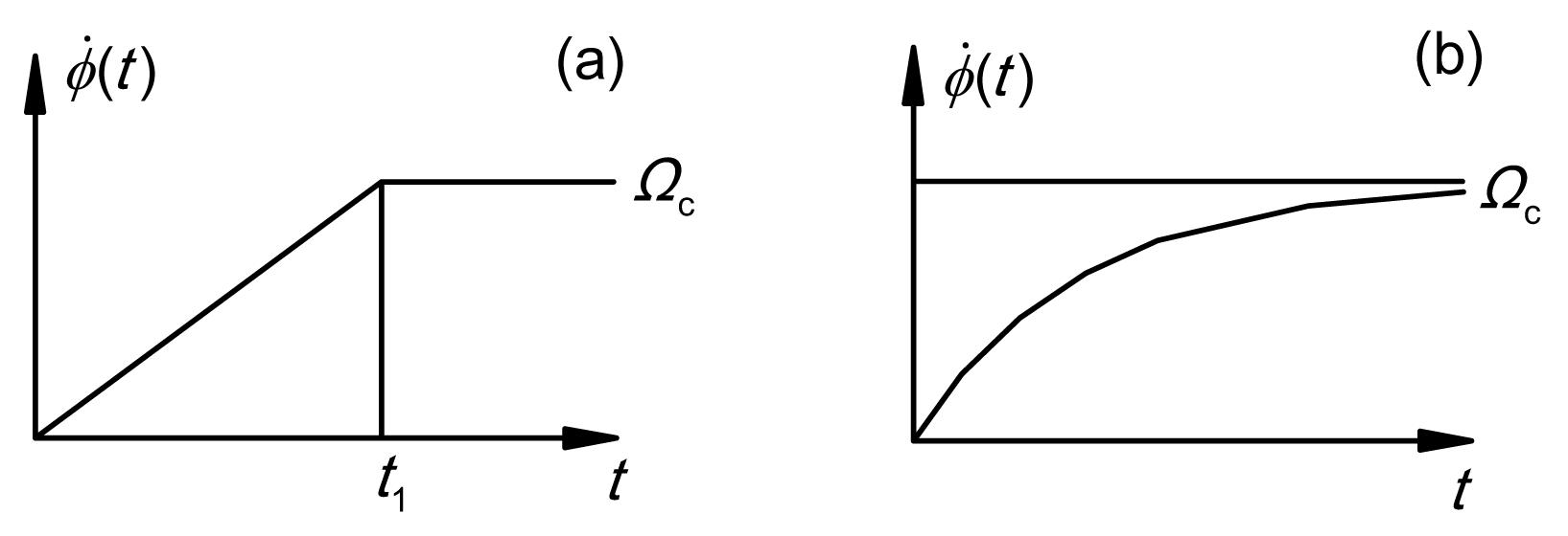
 In industrial applications, two laws of rising speed are of interest (Fig. 8), namely, the linear law and the exponential law (Lalanne and Ferraris, 1990).




 For the linear law: (40) (41) (42) where α is the angular acceleration.

 For the exponential law: (43) , (44) , (45) .

 Due to the existence of angular acceleration, the excitation forces caused by unbalance mass become more complicated during transient motion, and the expression is (46) .

5.  Numerical examples

 To demonstrate the application and accuracy of the proposed program, simulation on a typical dual rotor system was carried out to determine the critical speed and transient response. Fig. 7 outlines the structure and the following Tables 1–3 list the detailed parameters.










 There are two operation modes in dual rotor systems: co-rotation and counter-rotation. The speed ratio is in co-rotation, and in counter-rotation.

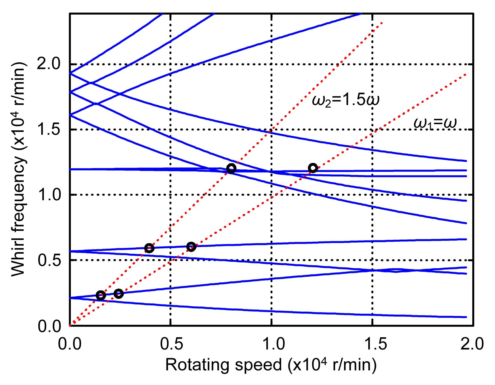
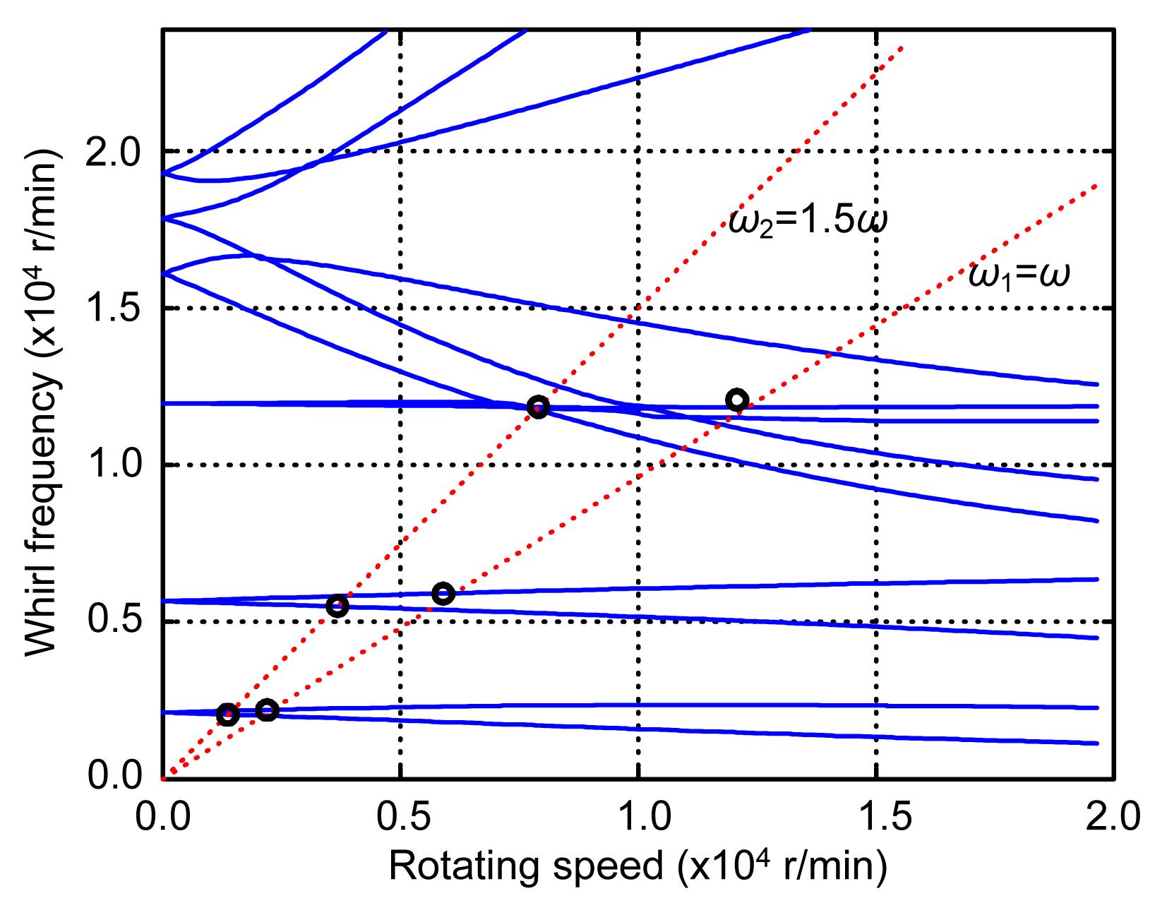
 Gyroscopic moments are related to the direction of rotation, so research on the dynamic characteristics in both co-rotation and counter-rotation was conducted. Campbell diagrams of these two cases were obtained by calculation of natural frequencies. Figs. 9 and 10 show the variation in whirl frequency with inner rotor speed when r_ω =1.5 and r_ω =−1.5, respectively.







 Table 4 lists the data for the corresponding intersections. Because the influence of gyroscopic moments on dual rotor structures may decrease in counter-rotation, the critical speeds are smaller.




 One common phenomenon that can be found in Figs. 9 and 10 is that the third order frequencies of both forward and backward whirl barely vary with rotation speed, while those of other orders vary significantly. In this specific case, this phenomenon indicates that the third order frequencies depend primarily on the bearing stiffness, while those of other orders depend more on the stiffness of the rotors.

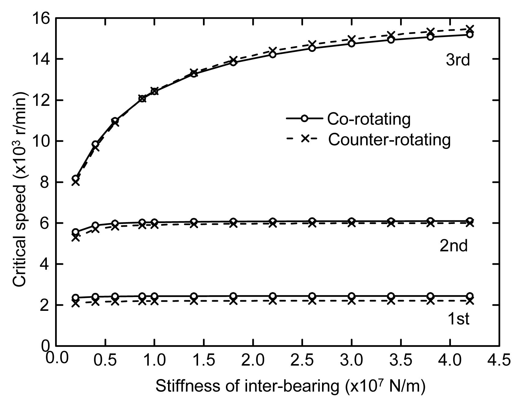
 In general, the stiffness of supports has a great effect on vibration performance; the inter-bearing stiffness, especially, is one of the key design parameters of a dual rotor system. The critical speeds of the first three orders were calculated with a set of such parameters, and the results are plotted in Fig. 11. The critical speeds of the first two orders are practically constant, while that of the third order increases. Furthermore, when counter-rotating, the critical speeds become more sensitive to the inter-bearing stiffness.




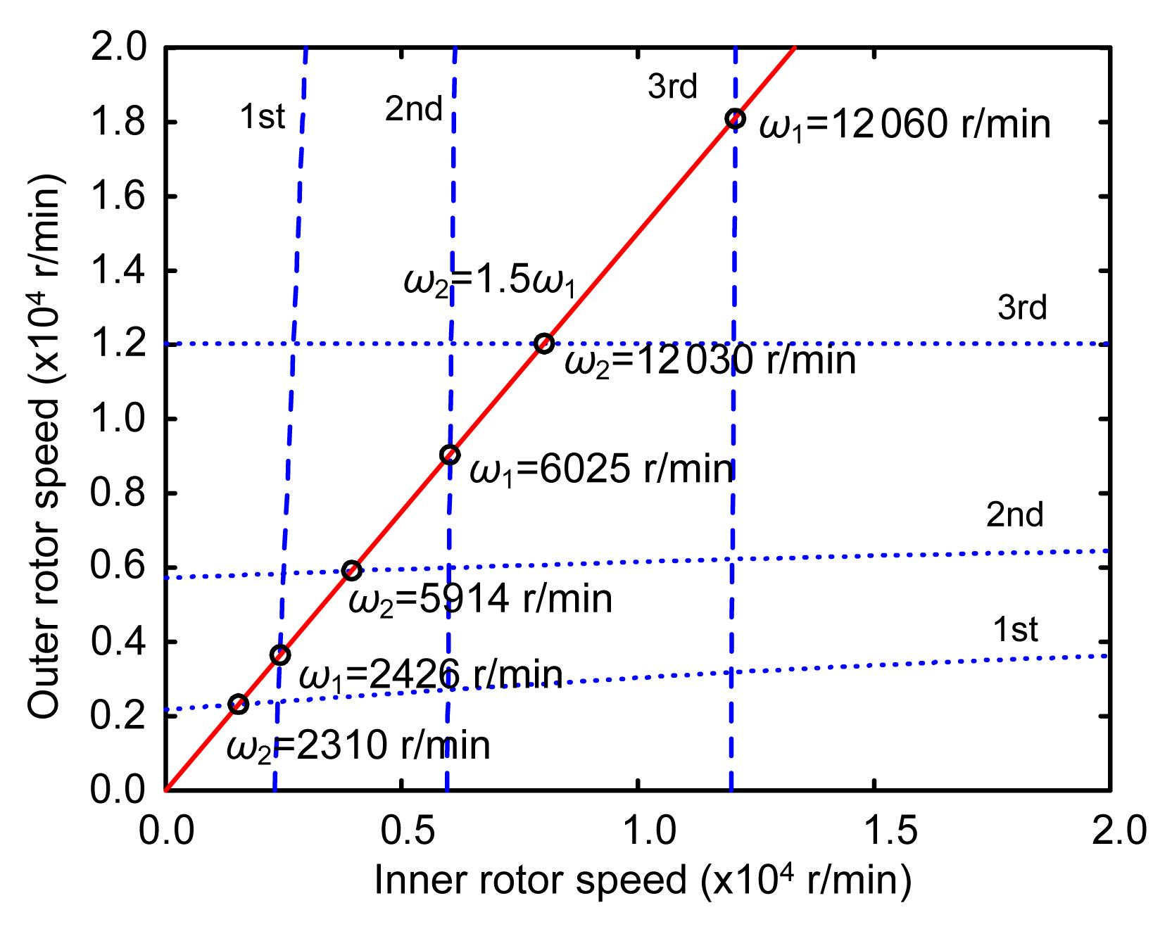
 A scanning calculation was carried out to find the resonant speeds of different rotating modes. Holding ω ₁ at a constant value while varying ω ₂, the corresponding critical speeds can be obtained from the Campbell diagrams (Table 5). Similarly, another group of data can be obtained with varying ω ₁ and fixed ω ₂. The critical speed map of the dual rotor system is drawn according to these two sets of results.




 In Fig. 12, the data for the intersections when r_ω =1.5 are approximately equal to those listed in Table 4. For the benefit of predicting resonance points, this kind of map is very helpful for choosing r_ω during the design process. It can be seen from the map or Table 5 that the speed ratio has almost no influence on the third order critical speed. The above analysis and the conclusion from Fig. 11 make it clear that the bearing stiffness has a significant impact on the natural frequencies of some specific orders.




 Transient simulation was carried out to examine the dynamic characteristics when a rotor system starts up and goes through the resonance region with different laws of rising speed. The parameters used were: simulation time: 0–6 s, time step: 0.0004 s, damping coefficient: β _c=0.001, unbalance mass on node 5: f _u=m _u e=50 g·mm.

 For the linear law:

 For the exponential law: .

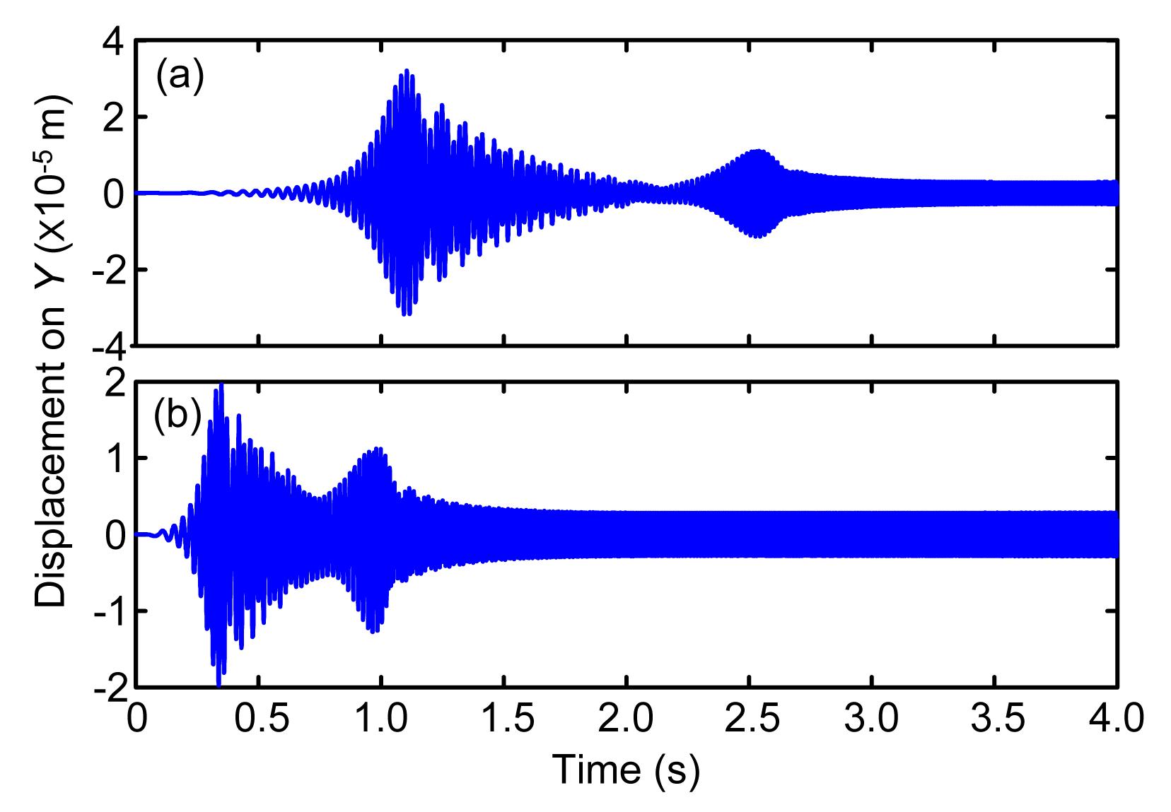
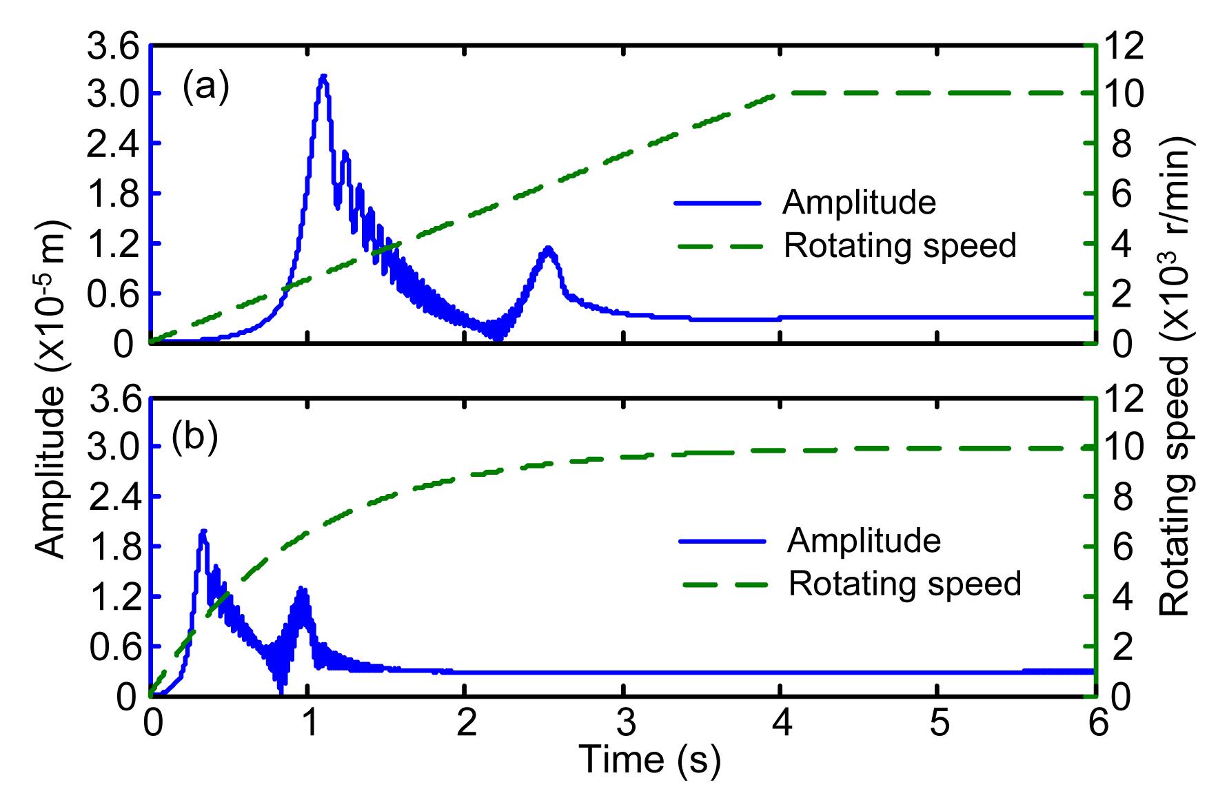
 The two sets of data in Fig. 13 are displacements of node 5 in the Y direction, corresponding to the linear and exponential laws, respectively. Similarly, the results in Fig. 14 are the transient amplitude. In practice, the exponential law is applied mostly for passing through the resonance region smoothly, as shown in the figure. Transient analysis can also be used to evaluate the stability of systems.







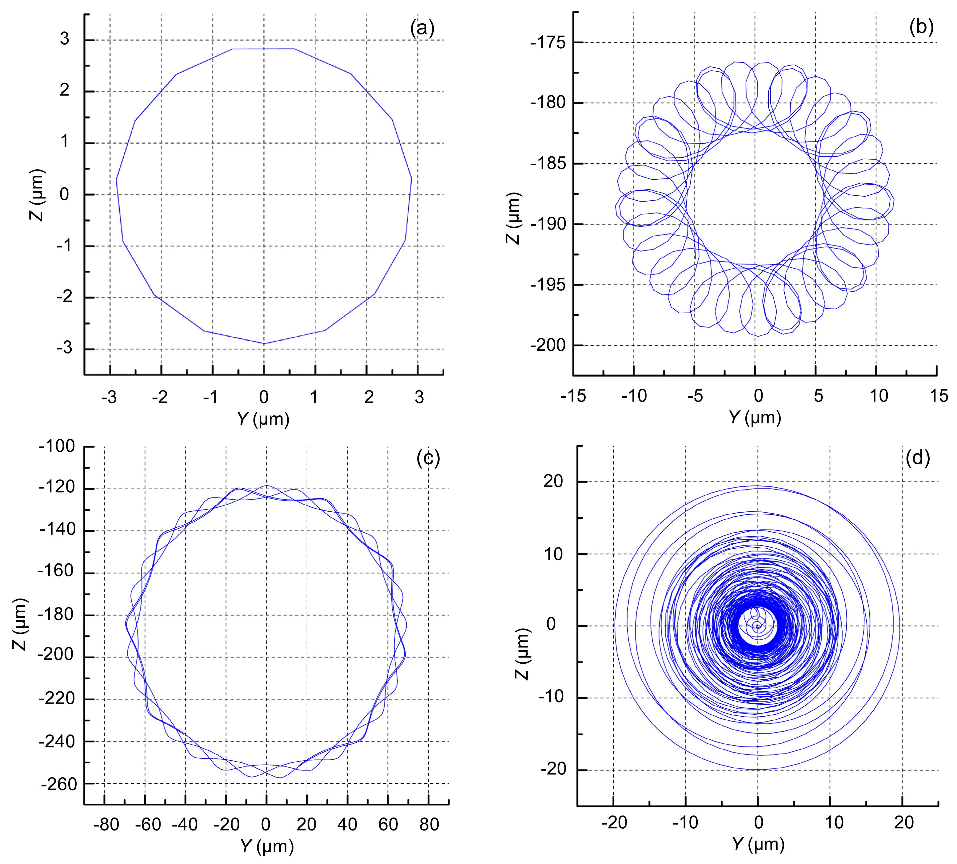
 The whirl orbit is one of the most important features for representing the motion state and it is the essential theme in the time domain analysis of vibration signals. To investigate the influence of different damping coefficients, the laws of rising speed and the gravity effect, the following simulations were completed. The particular conditions are listed in Table 6. Four trajectory diagrams of node 5 are illustrated in Fig. 15. Figs. 15a and 15b present the whirl behavior with and without, respectively, the gravity considered. Figs. 15b and 15c indicate that β _c affects the amplitude response explicitly. Fig. 15d shows the orbit of the entire start-up, showing that the stabilization occurs after passage through the critical speed.

6.  Conclusions

 The vibration equation of a dual rotor system was derived in detail, and by combining it with the Newmark method, a capable and efficient program was developed to solve its natural frequencies and simulate the transient response. FEM is practicable and effective for the engineering analysis of dual rotor systems, because the motion equations of subsystems can be coupled conveniently.

 Gyroscopic moments will lead to different critical speeds in co-rotation and counter-rotation. During counter-rotation, the critical speeds decrease since the gyroscopic moments will be partially canceled.

 The speed ratio r_ω will affect the dynamic characteristics of dual rotor system. A scanning calculation can be applied to draw a critical speed map, which is helpful for choosing this parameter during the design process.

 From the analysis of the transient response, we found that the exponential law was better than the linear law because of the smaller amplitude. The stability of the rotor bearing system can also be estimated by the orbits.

Appendix

References

[1] Abduljabbar, Z., ElMadany, M.M., AlAbdulwahab, A.A., 1996. Active vibration control of a flexible rotor. Computers and Structures, 58(3):499-511.
[2] Adhikari, S., 1999. Modal analysis of linear asymmetric non-conservative systems. Journal of Engineering Mechanics, 125(12):1372-1379.
[3] Adhikari, S., 2000. On symmetrizable systems of second kind. ASME Journal of Applied Mechanics, 67(4):797-802.
[4] Bathe, K.J., 1996. Finite Element Procedures. Prentice-Hall Inc.,New Jersey :768-784.
[5] Carrella, A., Friswell, M.I., Zotov, A., Ewins, D.J., Tichonov, A., 2009. Using nonlinear springs to reduce the whirling of a rotating shaft. Mechanical Systems and Signal Processing, 23(7):2228-2235.
[6] Das, A.S., Nighil, M.C., Dutt, J.K., Irretier, H., 2008. Vibration control and stability analysis of rotor-shaft system with electromagnetic exciters. Mechanism and Machine Theory, 43(10):1295-1316.
[7] Friswell, M.I., Dutt, J.K., Adhikari, S., Lees, A.W., 2010. Time domain analysis of a viscoelastic rotor using internal variable models. International Journal of Mechanical Sciences, 52(10):1319-1324.
[8] Garadin, M., Kill, N., 1983. A new approach to finite element modeling of flexible rotors. Engineering Computations, 1(1):52-64.
[9] Chiang, H.W.D., Hsu, C.N., Jeng, W., 2002. Turbomachinery Dual Rotor-Bearing System Analysis. ASME Turbo Expo 2002: Power for Land, Sea, and Air, Amsterdam, the Netherlands :803-810.
[10] Jei, Y.G., Lee, C.W., 1988. Finite element model of asymmetrical rotor-bearing systems. Journal of Mechanical Science and Technology, 2(2):116-124.
[11] Lalanne, M., Ferraris, G., 1990. Rotor Dynamics Prediction in Engineering. Wiley,New York :77-116.
[12] Lee, A.S., Ha, J.W., Choi, D.H., 2003. Coupled lateral and torsional vibration characteristics of a speed increasing geared rotor-bearing system. Journal of Sound and Vibration, 263(4):725-742.
[13] Nelson, H.D., 1980. A finite rotating shaft element using Timoshenko beam theory. ASME Journal of Mechanical Design, 102(4):793-803.
[14] Nelson, H.D., Mc-Vaugh, J.M., 1976. The dynamics of rotor-bearing systems using finite elements. ASME Journal of Engineering for Industry, 98(2):593-600.
[15] Newmark, N.M., 1959. A method of computation for structural dynamics. ASCE Journal of Engineering Mechanics, 85(3):67-94.
[16] Rajan, M., Nelson, H.D., Chen, W.J., 1986. Parameter sensitivity in the dynamics of rotor-bearing systems. ASME Journal of Vibration, Acoustics, Stress, and Reliability in Design, 108(2):197-206.
[17] Rao, J.S., 1996. Rotor Dynamics (3rd Ed.). New Age International Publishers,London :69-106.
[18] Rao, J.S., Shiau, T.N., Chang, J.R., 1998. Theoretical analysis of lateral response due to torsional excitation of geared rotors. Mechanism and Machine Theory, 33(6):761-783.
[19] Shiau, T.N., Rao, J.S., Chang, J.R., Choi, S.T., 1999. Dynamic behavior of geared rotors. ASME Journal of Engineering for Gas Turbines and Power, 121(3):494-503.
[20] Zhong, Y.E., 1987. Rotor Dynamics. (in Chinese), Tsinghua University Press,Beijing, China :176-195.
Open peer comments: Debate/Discuss/Question/Opinion