Liang Ling, Xin-biao Xiao, Jia-yang Xiong, Li Zhou, Ze-feng Wen, Xue-song Jin. A 3D model for coupling dynamics analysis of high-speed train/track system[J]. Journal of Zhejiang University Science A, 2014, 15(12): 964-983.
@article{title="A 3D model for coupling dynamics analysis of high-speed train/track system", author="Liang Ling, Xin-biao Xiao, Jia-yang Xiong, Li Zhou, Ze-feng Wen, Xue-song Jin", journal="Journal of Zhejiang University Science A", volume="15", number="12", pages="964-983", year="2014", publisher="Zhejiang University Press & Springer", doi="10.1631/jzus.A1400192" }
%0 Journal Article %T A 3D model for coupling dynamics analysis of high-speed train/track system %A Liang Ling %A Xin-biao Xiao %A Jia-yang Xiong %A Li Zhou %A Ze-feng Wen %A Xue-song Jin %J Journal of Zhejiang University SCIENCE A %V 15 %N 12 %P 964-983 %@ 1673-565X %D 2014 %I Zhejiang University Press & Springer %DOI 10.1631/jzus.A1400192
TY - JOUR T1 - A 3D model for coupling dynamics analysis of high-speed train/track system A1 - Liang Ling A1 - Xin-biao Xiao A1 - Jia-yang Xiong A1 - Li Zhou A1 - Ze-feng Wen A1 - Xue-song Jin J0 - Journal of Zhejiang University Science A VL - 15 IS - 12 SP - 964 EP - 983 %@ 1673-565X Y1 - 2014 PB - Zhejiang University Press & Springer ER - DOI - 10.1631/jzus.A1400192
Abstract: A 3D dynamic model of a high-speed train coupled with a flexible ballast track is developed and is presented in this study. In this model, each vehicle is modeled as a 42 degrees of freedom multi-body system, which takes into consideration the nonlinear dynamic characteristics of the suspensions. A detailed inter-vehicle connection model including nonlinear couplers and inter-vehicle dampers, and the linear tight-lock vestibule diaphragm is established to simulate the effect of the end connections of neighboring vehicles on dynamic behavior. The track is modeled as a traditional three-layer discrete elastic support model. The rails are assumed to be Timoshenko beams supported by discrete sleepers. Each sleeper is treated as an Euler beam and the ballast bed is replaced by equivalent rigid ballast bodies. The reliability of the present model is then validated through a detailed numerical simulation comparison with the commercial software SIMPACK, with the effect of the track flexibility on the train/track interaction being analyzed simultaneously. The proposed model is finally applied to investigate the difference between dynamic performances obtained using the entire-train/track model (TTM) and the single-vehicle/track model (VTM). Several key dynamic performances, including vibration frequency response, ride comfort, and curving performance, calculated by the two types of dynamic models are compared and discussed. The numerical results show that there is a significant difference between the dynamic behaviors obtained by VTM and TTM, and that inter-vehicle connections have an important influence on the dynamic behavior of high-speed vehicles.
Darkslateblue:Affiliate; Royal Blue:Author; Turquoise:Article
Article Content
1. Introduction
High-speed railways are developing rapidly in many countries around the world. The mileage of commercial high-speed railway in China now exceeds 6000 km. The operating speed of high-speed trains ranges from 200 km/h to 350 km/h. China plans to construct 16 000–18 000 km of passenger dedicated lines by 2020, with operating speeds exceeding 200 km/h (Zhang, 2009). Nowadays more and more people consider high-speed trains as a comfortable, safe, low emission, and clean energy consumption transportation tool with a high on-schedule rate. But increasing the speed posts very high requirements in service performance, running safety, and vibration control in environments which are all closely related to the dynamic performance of the train/track coupling system. Therefore, the following studies on train/track system dynamics are very important for designing well matched high-speed trains/tracks and ensuring the safe operation of high-speed trains.
Railway system dynamics studies have been performed for almost a century, resulting in thousands of papers and theoretical models being published (Knothe and Grassie, 1993; Popp et al., 1999; Evans and Berg, 2009; Zhai et al., 2009; Arnold et al., 2011; Xiao et al., 2014). Throughout previous studies, there are mainly two types of simulation models: single-vehicle/track coupling models and models for multi-vehicles (or trains) coupled with a rigid or nearly rigid track.
In traditional railway vehicle dynamics simulations and track modeling using commercial software, such as SIMPACK, NUCARS, GENSYS, and VAMPIRE, the railway track is often assumed to be a rigid or nearly rigid structure. However, many studies have pointed out that track flexibility has a significant influence on wheel-rail contact behavior and vehicle/track dynamics. Neglecting track dynamic behavior may lead to a significant overestimation of railway vehicle dynamic performance, including hunting stability, wheel-rail contact forces, and other vehicle system dynamical behaviors that are involved (Jin et al., 2002; Zhai et al., 2009; Di Gialleonardo et al., 2012). In addition, the classical vehicle dynamics study using a simplified rigid track model cannot solve the dynamic problems caused by the failure of a track component and other severe conditions, such as the running safety of railway vehicles passing over unsupported tracks, broken rails, and buckled tracks. These models, of course, cannot characterize the dynamical behavior of track components or the ground vibration induced by high-speed trains in operation. Another important factor to consider is that a train running on a track is a large-scale coupling system, and that the dynamic behaviors of the train and the track, and the neighboring vehicles significantly affect each other. Thus, it is necessary to develop a 3D dynamic model of a high-speed train coupled with a flexible track to allow a deeper investigation into the dynamical behavior of high-speed trains under various conditions. That is the purpose of the present study.
The widely used coupled single-vehicle/track models (VTMs) can simulate the basic phenomena of a vehicle coupled with a track. An overview of single-vehicle/track modeling and its interaction analysis can be seen in (Knothe and Grassie, 1993; Popp et al., 1999; Zhai et al., 2009). Most of the existing models were used to deal with single-vehicle/track vertical interaction problems (Nielsen and Igeland, 1995; Fröhling, 1998; Oscarsson and Dahlberg, 1998; Sun and Dhanasekar, 2002; Lei and Mao, 2004; Cai et al., 2008), and a few were used to analyze lateral and vertical dynamical behavior (Zhai et al., 1996; Sun et al., 2003; Jin et al., 2006; Baeza and Ouyang, 2011; Xiao et al., 2011; Zhou and Shen, 2013). In addition, a few models for train/railway structure interactions were developed to investigate railway system dynamics (Yang and Wu, 2002; Xia et al., 2003; Tanabe et al., 2008; Ju and Li, 2011).
Although coupled VTMs can solve many scientific problems effectively, there are some issues which these models cannot deal with. The most prominent one is that they cannot consider the effect of inter-vehicle connections in the dynamic behavior of the train/track system. Most modern high-speed trains are equipped with tight-lock inter-vehicle connections, such as tight-lock couplers and inter-vehicle dampers. When high-speed trains run in complex operating environments, such as a derailment occurring due to strong cross-winds, earthquakes, or serious track buckling, the mutual influence between the adjacent vehicles on the system’s dynamic behavior should not be neglected in a dynamical behavior analysis (Evans and Berg, 2009; Zhang, 2009; Jin et al., 2013). In these environments, any VTM cannot characterize the behavior of the vehicle and track accurately and reliably. To the authors’ knowledge, no previous research results have been published regarding the difference between the dynamical behaviors calculated by using a VTM and an entire-train/track model (TTM) even when a train operates under normal conditions. In the present investigation, the differences in several key dynamic behaviors between these two types of dynamic models are clarified.
To meet the challenges of the various complex dynamics problems of high-speed trains coupled with tracks, the existing models need to be further improved in two ways: the space scale of trains coupled with tracks and the modeling of their key components. In this study, a 3D dynamic model of a high-speed train coupled with a ballast track is developed, which extends the single-vehicle/track vertical-lateral coupling model to a multi-vehicle/track vertical-lateral-longitudinal coupling model. In the 3D coupled train/track model, each vehicle is modeled as a 42 degrees of freedom (DOFs) multi-body system, which considers the nonlinear dynamic characteristics of the suspension systems and the longitudinal motion of the vehicle components. To simulate the interaction between adjacent vehicles, a detailed inter-vehicle connection model is developed, which considers nonlinear couplers, nonlinear inter-vehicle dampers, and a linear tight-lock vestibule diaphragm. The track is a flexible 3-layer model consisting of rails, sleepers, and ballast. The dynamic behavior and elastic structure of the track components are considered. An improved wheel/rail contact geometry model is introduced to take the effect of the profiles and the instant deformation of the wheel and the rail into account (Chen and Zhai, 2004; Xiao et al., 2011). The modified model is also able to deal with separation occurring between the wheels and the rails. A moving sleeper support track model is adopted to simulate train/track excitation caused by the discrete sleepers (Xiao et al., 2011). The reliability of the 3D coupled train/track model is then validated through a detailed numerical comparison with the commercial software, SIMPACK, and the contrast caused by different track modeling methods is analyzed. Also, the differences are investigated between the dynamical behaviors obtained by VTM and TTM, with the results calculated using the proposed TTM being more reasonable. The investigated dynamical behaviors include vibration frequency components, ride comfort, and curving performance, which are important in estimating the operational qualities and dynamic characteristics of trains and tracks.
2. 3D modeling of high-speed train/track system
A 3D dynamic model of a high-speed train coupled with a ballast track is developed in this study (Fig. 1). The coupled train/track dynamic model consists of four subsystems: the vehicle, the inter-vehicle connection, the track, and the wheel/rail contact. The interaction of the vehicles and the track is characterized through the wheels/rails in rolling contact, and the interaction between adjacent vehicles is transferred via the inter-vehicle connection. They are described in Sections 2.1, 2.2, 2.3, and 2.4 in detail.
Fig.1 High-speed train/track coupling model
2.1. Modeling vehicle subsystem
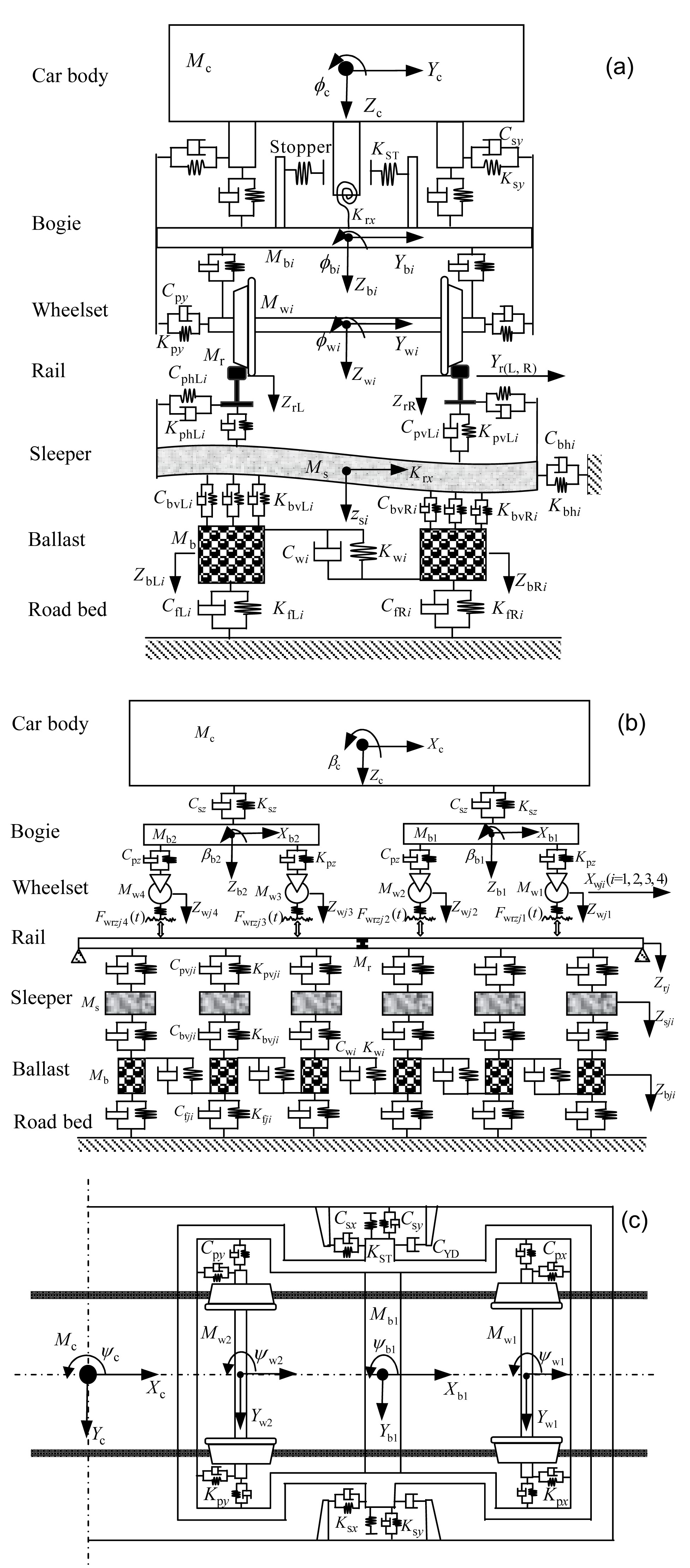
A new generic Chinese high-speed train, named CRH380A, is selected to be modeled in this study. The train consists of six power vehicles and two trailing vehicles, and its highest operating speed reaches 380 km/h. The calculation model of a high-speed vehicle coupled with a ballast track is shown in Fig. 2. In the coupled dynamic model, each power vehicle or each trailing vehicle is modeled as a 42 DOFs nonlinear multi-body system, which includes seven rigid components: a car body, two bogies, and four wheelsets.
Fig.2 3D views of the vehicle and track model: (a) elevation; (b) side elevation; (c) planform
In Fig. 2, the coordinate system x-y-z is a Cartesian system and the initial one. Axis x is in the moving direction of the high-speed train, axis z is in the vertical direction, and axis y is in the lateral direction of the track. For convenience, the front bogie and the rear bogie are numbered 1 and 2, respectively; the leading wheelset and the trailing wheelset of the front bogie are numbered as 1 and 2, respectively; and the corresponding wheelsets of the rear bogie are indicated by 3 and 4, respectively. The subscript j (j=L or R) refers to the left or right side when looking in the direction of movement of the train. Each component of the vehicle has six DOFs: the longitudinal displacement X, the lateral displacement Y, the vertical displacement Z, the roll angle ϕ, the pitch angle β, and the yaw angle ψ. In Fig. 2, the notations C and K with subscripts stand for the coefficients of the equivalent dampers and the stiffness coefficients of the equivalent springs, respectively. The equivalent dampers and springs are used to replace the connections between the components of the high-speed vehicle and the ballast track.
The equations of motion of the car body in the longitudinal, lateral, vertical, rolling, pitching, and yawing directions are
where Mc is the mass of the car body; Icx, Icy, Icz are the rolling, pitching, and yawing moments of inertia, respectively; and are the accelerations of the car body center in the longitudinal, lateral, vertical, rolling, pitching, and yawing directions, respectively; is the angular deflection of the car body rolling caused by the cant of the high rail; Fxsi, Fysi, Fzsi, Mxsi, Mysi, and Mzsi (i=1, 2) denote the mutual forces and moments between car body and bogie frames in the x, y, and z directions; subscripts 1 and 2 indicate the front and rear bogies; Fxci, Fyci, Fzci, Mxci, Myci, and Mzci (i=f or b) denote the inter-vehicle forces and moments caused by inter-vehicle connections between the adjacent car bodies in the x, y, and z directions; and subscripts f and b indicate the front and end of each car body. Detailed expressions of the inter-vehicle forces between the adjacent vehicles will be given in Section 2.2. Fycc, Fzcc, Mxcc, and Mzcc denote the external forces on the car bodies resulting from the centripetal acceleration when a train is negotiating a curved track. Lastly, g is the gravitational acceleration.
The equations of motion of the bogie i (i=1, 2), in the longitudinal, lateral, vertical, rolling, pitching, and yawing directions are
where Mb is the mass of the bogie; Ibx, Iby, and Ibz are the moments of inertia of the bogie in rolling, pitching, and yawing motions; and are the accelerations of the bogie center in the longitudinal, lateral, vertical, rolling, pitching, and yawing directions, respectively; is the angular deflection of the bogie rolling caused by the cant of the high rail; Fxfi, Fyfi, Fzfi, Mxfi, Myfi, and Mzfi (i=1, 2, 3, 4) denote the mutual forces and moments between bogie frames and wheelsets in the x, y, and z directions; subscripts 1, 2, 3, 4 indicate the four wheelsets of the vehicle, respectively; and Fycbi, Fzcbi, Mxcbi, and Mzcbi (i=1, 2) denote the external forces on bogies resulting from the centripetal acceleration when the vehicle is negotiating curved track.
The equations of motion of the wheelset i (i=1, 2, 3, 4) in the longitudinal, lateral, vertical, rolling, pitching, and yawing directions are
where Mw is the mass of the wheelset; Iwx, Iwy, and Iwz are the moments of inertia of the wheelset in rolling, pitching, and yawing motions, respectively; and are the accelerations of the wheelset in the longitudinal, lateral, and vertical directions, respectively; and are the angular accelerations in rolling, spin, and yawing directions, respectively; is the angular deflection of the wheelset rolling caused by the cant of the high rail; Fwrxi, Fwryi, Fwrzi, Mwrxi, Mwryi, and Mwrzi (i=1, 2, 3, 4) denote the contact forces and moments between the wheels and the rails in the x, y, and z directions, respectively; Fycwi, Fzcwi, Mxcwi, and Mzcwi (i=1, 2, 3, 4) denote the external forces on the wheelsets resulting from the centripetal acceleration when the train is negotiating curved track; and MTBi is the traction or braking moment acting on the wheelsets when the train is accelerating or decelerating. In this study, a constant traveling speed of the train is assumed. Thus, MTBi equals zero here.
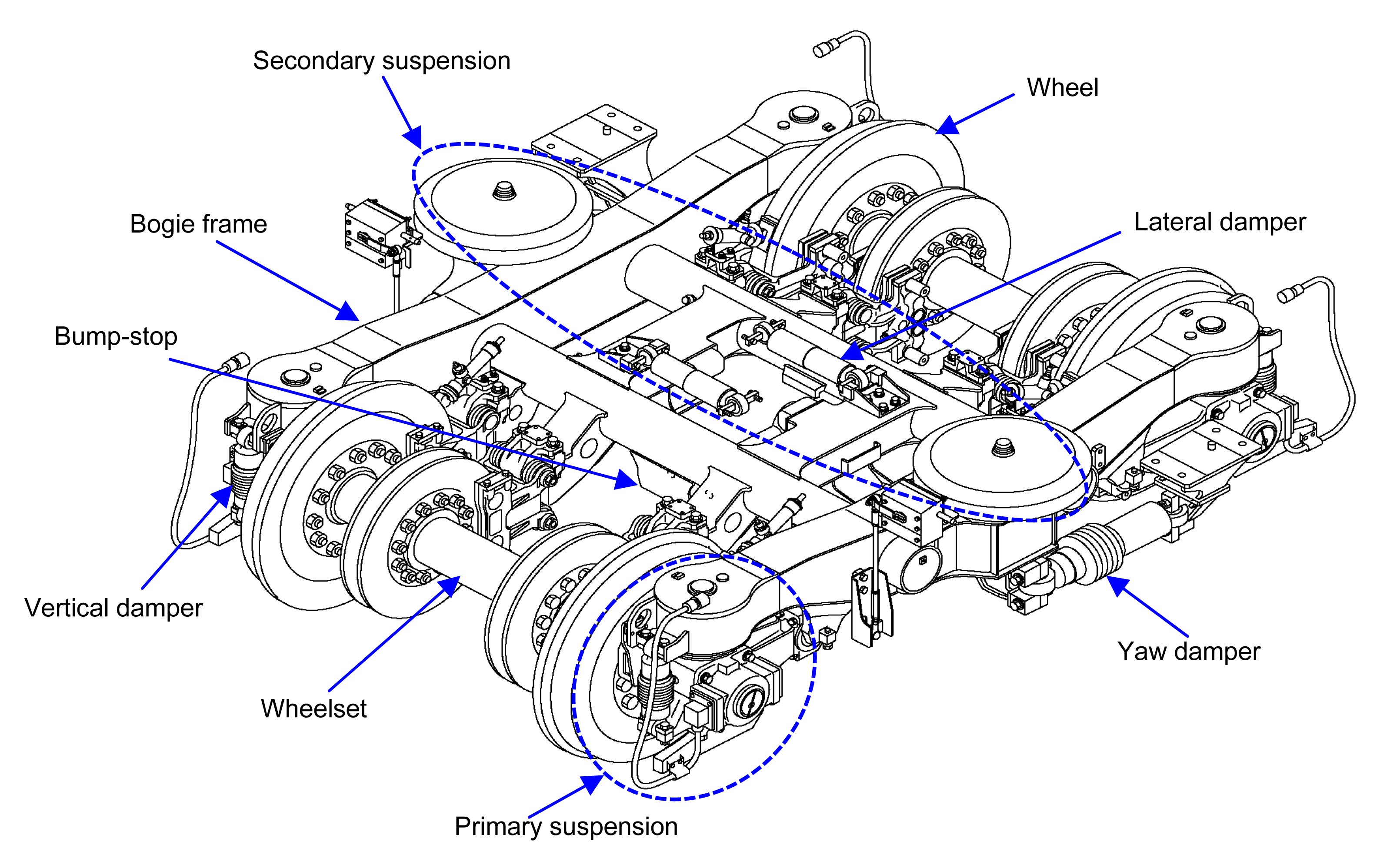
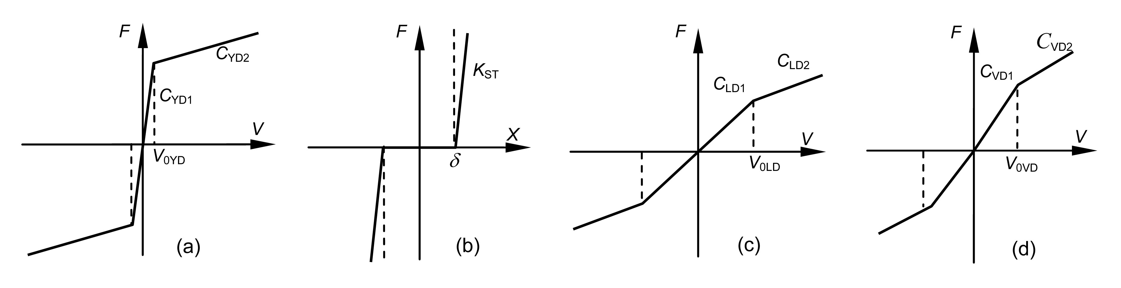
In the present train/track model, each bogie is equipped with double suspension systems. The wheelsets and the bogies are connected by the primary suspensions, while the car body is supported on the bogies through the secondary suspensions. The primary and secondary suspension systems were represented using 3D spring-damper elements, and the nonlinear dynamic characteristics of the suspension systems were considered. The nonlinear suspension elements include the yaw and lateral dampers and the bump-stops installed on the secondary suspension, and the vertical dampers installed on the primary suspension, as illustrated in Fig. 3. In the model developed in this study, the nonlinear behavior of the suspension system components was modeled using bilinear spring and damping elements, as shown in Fig. 4.
Fig.3 Bogie of a Chinese high-speed train
Fig.4 Nonlinear characteristics of the vehicle suspensions (a) Yaw damper; (b) Bump-stop; (c) Lateral damper; (d) Vertical damper
According to the bilinear postulation, the forces between the bogies and the car body or the wheelsets are
where CYD, CLD, and CVD stand for the equivalent coefficients of the yaw dampers, the lateral dampers, and the vertical dampers, respectively; KST is the contact stiffness when the car body is contact with the bump-stops; V0YD, V0LD, V0VD are the load-off velocities of the yaw dampers, the lateral dampers, and the vertical dampers, respectively; δ is the lateral clearance between the car body and the bump-stops on the bogie frames; is the longitudinal relative velocity between the car body and the side frame; is the lateral relative displacement between the bottom of the car body and the bogies; is the lateral relative velocity between the bottom of the car body and the bogies; is the vertical relative velocity between the axle and the side frame; FxYD, FyST, FyLD are the forces of the yaw dampers, the bump-stops, and the lateral dampers between bogies and car body, respectively; and FzVD is the force of the vertical dampers between bogies and wheelsets.
2.2. Modeling the inter-vehicle connection subsystem
The design of the inter-vehicle connection is very important for a high-speed train because it has to include mechanical and electrical connections between adjacent vehicles. In addition, it should provide passengers with a comfortable and safe passage. Among the inter-vehicle suspensions of a high-speed train, three devices have a significant influence on the dynamics of the train/track system: couplers, inter-vehicle dampers, and tight-lock vestibule diaphragms. In the present model, the nonlinear couplers and inter-vehicle dampers are replaced with nonlinear spring-damper elements and are retractable only along the axial direction. The tight-lock vestibule diaphragm is simplified as a linear 3D spring element, which can restrain the adjacent vehicles in the longitudinal, lateral, vertical, rolling, pitching, and yawing directions. Therefore, the inter-vehicle forces can be calculated based on the deformation of the connectors and the relative angles between connectors and car bodies.
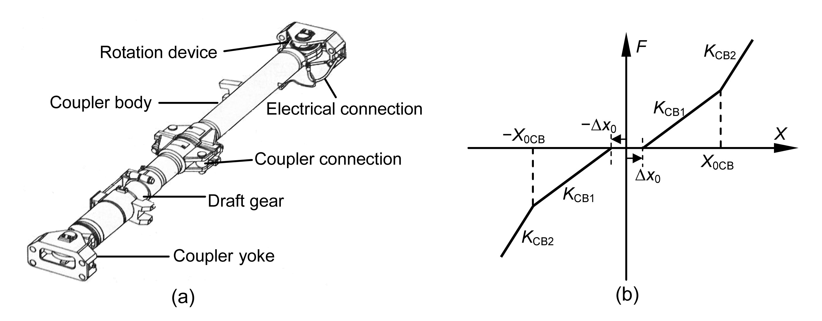
To improve running stability and ride comfort during acceleration or deceleration, tight-lock couplers are installed comprehensively on modern high-speed trains. A type of tight-lock coupler system used on the Chinese high-speed trains is modeled in this study, as shown in Fig. 5a. In this type of tight-lock coupler, the couplers installed on adjacent vehicles are fixed by the coupler connection, and the slackless is very small. The couplers can rotate by a certain angle around the coupler yoke in the horizontal and vertical directions. The coupler body is approximately rigid, and the inter-vehicle contact stiffness is offered by the draft gear. In this model, the nonlinear stiffness characteristic of the draft gear is considered, and the draft gear is modeled by a bilinear spring element, as shown in Fig. 5b. According to the bilinear assumption, the coupler forces are
where Δx is the relative displacement between the two ends of the couplers connecting the adjacent vehicles in the axial direction, Δx0 is the slackless of the coupler, X0CB is the initial length of the coupler, and KCB is its equivalent stiffness coefficient.
Fig.5 Nonliear coupler model (a) and nonlinear characteristic of coupler system (b)
According to the dynamic responses of the vehicles and the geometric relationship between couplers and car body ends, the lateral and vertical angles between the coupler and the adjacent vehicles can be calculated (Garg and Dukkipati, 1984). The longitudinal, lateral, and vertical components of the coupler forces applied to the adjacent vehicles near to the coupler are then obtained.
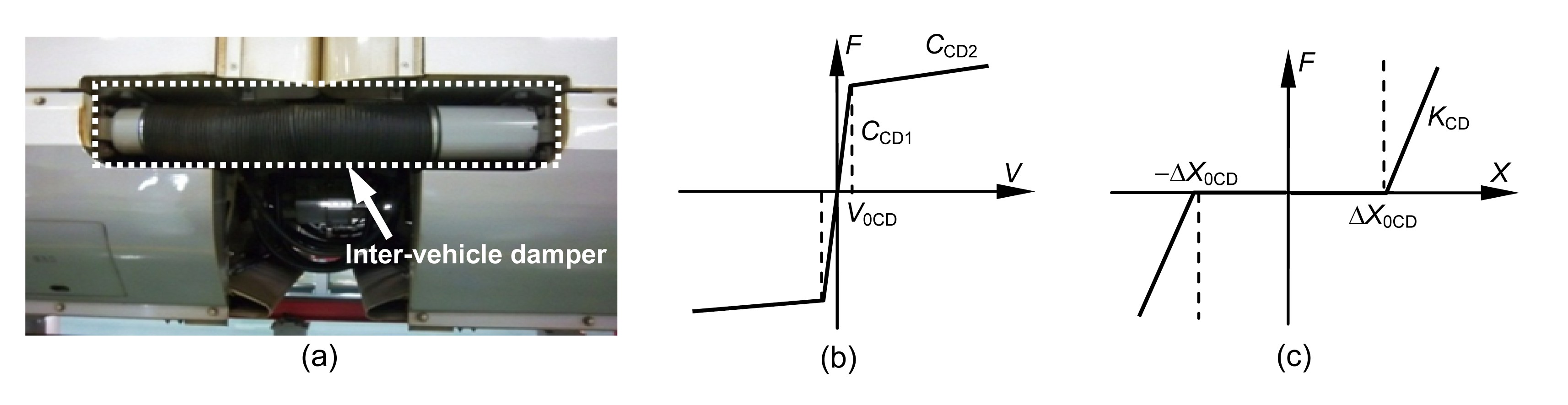
Inter-vehicle dampers are widely used on high-speed trains, such as the German ICE, the French TGV, the Japanese Shinkansen train sets, and the Chinese CRH. In the present model, a type of longitudinal inter-vehicle damper used on Chinese high-speed trains is introduced, as shown in Fig. 6a. Field tests and numerical studies (Zhang, 2009) highlight that this kind of damper can reduce the longitudinal impacts between the vehicles and improve the lateral stability and ride comfort of high-speed trains. The inter-vehicle dampers are also replaced with bilinear spring-damper elements, and their damping and stiffness are considered, as shown in Figs. 6b and 6c. Based on Fig. 6, the forces on the inter-vehicle dampers are
where FCDi (i=L, R) are the interaction forces of the longitudinal inter-vehicle dampers; CCD and KCD stand for the coefficients of the equivalent damper and the equivalent spring, respectively; V0CD is the load-off velocity of the inter-vehicle dampers; X0CD is the initial length of the inter-vehicle damper; ΔVCDi and ΔXCDi (i=L, R) are the relative velocity and displacement between two ends of the inter-vehicle dampers connecting adjacent vehicles in the axial direction, respectively; and the subscript i (i=L, R) refers to the left or right longitudinal inter-vehicle damper. Using the same process as in the coupler angle calculation, the relative angles between the dampers and the car body ends are then calculated. Thus, the forces caused by the inter-vehicle dampers in x, y, and z directions can be obtained.
The tight-lock vestibule diaphragm also has an impact on the dynamics of a high-speed train. For simplicity, it is replaced with 3D linear spring elements in the present model, which can supply the car body with restraining stiffness in the longitudinal, lateral, vertical, rolling, pitching, and yawing directions.
2.3. Modeling the track subsystem
The model of the track is a flexible one consisting of rails, sleepers, and ballasts, as shown in Fig. 2. In the track model, rails are assumed to be Timoshenko beams supported by discrete sleepers, and the effects of vertical and lateral motions, and rail roll on wheel/rail creepage are taken into account. Each sleeper is treated as an Euler beam supported by a uniformly distributed stiffness and damping in its vertical direction, and a lumped mass is used to replace the sleeper in its lateral direction. The ballast bed is replaced by equivalent rigid ballast bodies in the calculation model, taking into account only the vertical motion of each ballast body. The motion of the roadbed is neglected. The equivalent springs and dampers are used as the connections between rails and sleepers, between sleepers and ballast blocks, and between ballast blocks and the roadbed.
The bending deformations of the rails are described by the Timoshenko beam theory. Using the modal synthesis method and normalized shape functions of a Timoshenko beam, the fourth-order partial differential equations of the rails are converted into second-order ordinary differential equations as follows:
For the lateral bending motion:
For the vertical bending motion:
For the torsional motion:
In Eqs. (10)–(12), qryk(t), qrzk(t), and qrTk(t) are the generalized coordinates of the lateral, vertical, and rotational deflection of the rail, respectively, while wryk(t) and wrzk(t) are the generalized coordinates of the deflection curve of the rail with respect to the z-axis and the y-axis. The material properties of the rail are indicated by the density ρr, the shear modulus Gr, and Young’s modulus Er. mr is the mass per unit longitudinal length. The geometry of the cross section of the rail is represented by the area Ar, the second moments of area Iry and Irz around the y-axis and the z-axis, respectively, and the polar moment of inertia Ir0. The shear coefficients κry=0.4057 and κrz=0.5329 for the lateral and the vertical bending and the shear coefficient Kr=2.473 346×10−6 are obtained through a finite element analysis of the rail profile of Chinese CN 60 using the software package ANSYS. The calculation length of the beam is denoted by lr, the value of which was set at 420 m when considering an eight-vehicle train running on the calculated track. In this case, 1000 vibration modes of the rail were considered, and the frequency of the highest mode was approximately 1.2 kHz. Ryi and Rzi are the lateral and vertical forces between the rail and sleeper i, respectively. The wheel/rail forces at the wheel j in the lateral and vertical directions are represented by Fwryj and Fwrzj, respectively. Msi and MGj denote the equivalent moments acting on the rail. xsi and xwj denote the longitudinal positions of the sleeper i and the wheel j, respectively, and Nw and Ns are the number of wheelsets and sleepers within the analyzed rail, respectively. The subscript i indicates sleeper i, and j for wheel j. NMY, NMZ, and NMT are the total numbers of the shape functions, and Yrk(x), Zrk(x), and Φrk(x) are the kth shape functions, which are given by
,
,
.
The sleeper in the present model is treated as an Euler-Bernoulli beam with free-free ends in the vertical direction while a lumped mass is used to replace it for its lateral motion. The longitudinal rigid motion and rotating motion of each sleeper are neglected, as shown in Fig. 2. Using the modal synthesis method and the normalized shape functions of the Euler beam, the fourth-order partial differential equations of its vertical vibration can be simplified as a second-order ordinary differential equation as follows:
where qszk(t) are the generalized coordinates of the sleeper vertical deflection, Es is Young’s modulus, Is is the second moment of area of the sleeper cross-section about the y axis, ms is the mass per unit longitudinal length, ls is the length of the sleeper, Nb and Nr are the number of ballast and rails within the analyzed sleeper, respectively, Fbzi is the force between the sleeper and the ballast body in the action spot i, Rzj is the force between the sleeper and the rail in the action location j, NMS is the total number of the shape functions, and Zsk(y) is the kth modal function, which is given by
where αk and Ck are the frequency coefficient and the function coefficient of a beam with free-free boundary conditions, respectively.
The equation of the lateral rigid motion of the sleeper is
,
where FyLi and FyRi are the lateral forces between sleeper i and the left and right rails, and Fbyi is the equivalent lateral support force by the ballast body. The longitudinal rigid motion and rotating motion of each sleeper are neglected.
The ballast bed is replaced by equivalent rigid ballast blocks in this calculation model, while only the vertical motion of each ballast body is taken into account. The vertical equations of motion of the ballast body i are
,
,
where FzfLi, FzrLi, FzfRi, FzrRi, and FzLRi are the vertical shear forces between neighboring ballast bodies, FzgLi and FzgRi are the vertical forces between ballast bodies and the roadbed, and Mbs is the mass of each ballast body. Such a ballast model can represent the in-phase and out-of-phase motions of two vertical rigid modes in the vertical-lateral plane of the track. For brevity, the detailed derivation of track system equations, which can be seen in (Zhai et al., 2009; Xiao et al., 2011), are omitted here. Note that it is easy to develop the present track model in the case of a slab track or other ballastless tracks. The results for a slab track are not given here. A detailed description of the slab track model can be seen in (Xiao et al., 2012).
2.4. Modeling the wheel/rail contact subsystem
The wheel/rail contact is an essential element that couples the vehicle subsystem with the track subsystem. The wheel/rail contact model includes two basic issues: the geometric relationship and the contact forces between the wheel and the rail. The wheel/rail contact geometry calculation is necessary to acquire the location of the contact point on the wheel and rail surfaces, and the wheel/rail interaction forces. In this study, an improved geometric calculation model of the wheel/rail contact based on the method discussed in (Jin et al., 2005) is introduced. The modified spatial wheel/rail geometric contact model is able to take the instant motion and deformation of the rails into account and to deal with the separation of wheel and rail (Chen and Zhai, 2004; Xiao et al., 2011).
In this study, calculating the wheel/rail normal force uses the Hertzian nonlinear contact spring model, and the creep force calculation uses Shen et al. (1983)’s model based on Kalker (1967)’s linear creep theory. These two models are based on the assumptions of Hertzian contact theory. The contact points were previously calculated in the wheel/rail force calculation. The detail contact point calculation is described as follows.
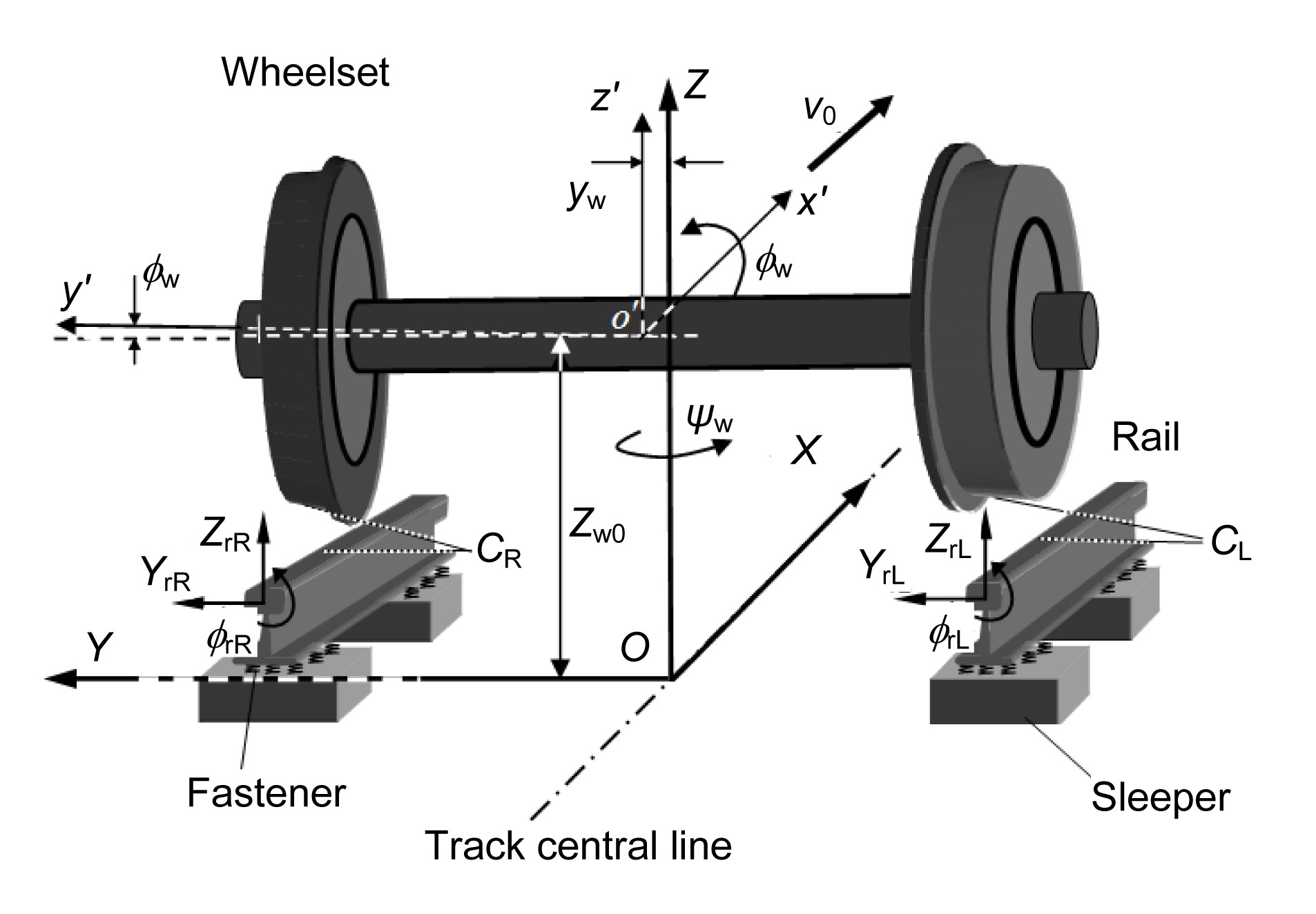
The wheel/rail contact points vary with the lateral displacement yw, yawing angle ψw, and rolling angle ϕw of the wheelset; the lateral displacements YrL,R, vertical displacements ZrL,R, and torsion angles ϕrL,R of the rail obtained through the dynamics calculation; and the given profiles of the wheel and rail. The profiles of the rails and wheels are expressed with the discrete datum, which is described in coordinate systems OXYZ and o′x′y′z′, respectively, as shown in Fig. 7. The origin of o′x′y′z′ is fixed at the center of the wheelset, and its axis y′ coincides with the axle of the wheelset. By solving the vehicle and track system equations, the instant motions of the wheelset and the two rails, and the positions of the rails at any given moment in a fixed reference configuration OXYZ are calculated, as shown in Fig. 7. In the contact geometry calculation, the height Zw0 of the wheelset in OXYZ is then set high enough to ensure no penetration occurred between the wheels and the rails. Using the wheel/rail contact point trace method (Wang, 1984), the minimum vertical distances between the wheels and the rails are calculated on both of the left and right sides. Hence, the two points on the wheel and rail treads with the smallest distance for each side wheel/rail are obtained, respectively. These two points constitute a pair of contact points CL,R between the wheelset and the two rails before their deformation.
Fig.7 Wheel/rail contact geometry calculation model
Using the known locations of the contact points, one obtains the curvature radii of the wheels/rails at their contact points according to the prescribed wheel/rail profiles. Using the radii and the static wheel normal load, one calculates the semi-axle lengths of the wheel/rail contact patches and the initial wheel/rail normal approach by means of Hertzian contact theory; then the Kalker (1967)’s creep coefficients can be found from his creep coefficient table. So far the calculation of the wheel/rail forces (normal and tangent) can be carried out by using the Hertzian contact nonlinear contact spring model and Shen et al. (1983)’s model.
The calculation model of the wheel/rail normal force, which characterizes the relationship law of the normal load and deformation between the wheel and rail, is described by a Hertzian nonlinear contact spring with a unilateral restraint, and reads
where G is the wheel/rail contact constant (m/N2/3), which can be obtained using the Hertzian contact theory. Zwrnc(t) is the normal compressing amount (or the normal approach) at the wheel/rail contact point. Zwrnc(t) is strictly defined as an approach between the two far points, one belonging to the wheel, and the other belonging to the rail. It can be determined by solving the system of equations and calculating the contact geometry of the wheelset and the rails discussed above. In Eq. (21), Zwrnc(t)>0 indicates the wheel/rail in contact, and Zwrnc(t)≤0 stands for their separation. The creep force calculation employs Shen et al. (1983)’s model, which is based on Kalker (1967)’s linear creep theory. Kalker (1967)’s linear creep theory is only available for small creepages. When large creepages are generated as, for example, in the case of wheel/rail flange contact, the creep force saturates, and then the creep forces vary nonlinearly with the creepages.
2.5. Train/track excitation model
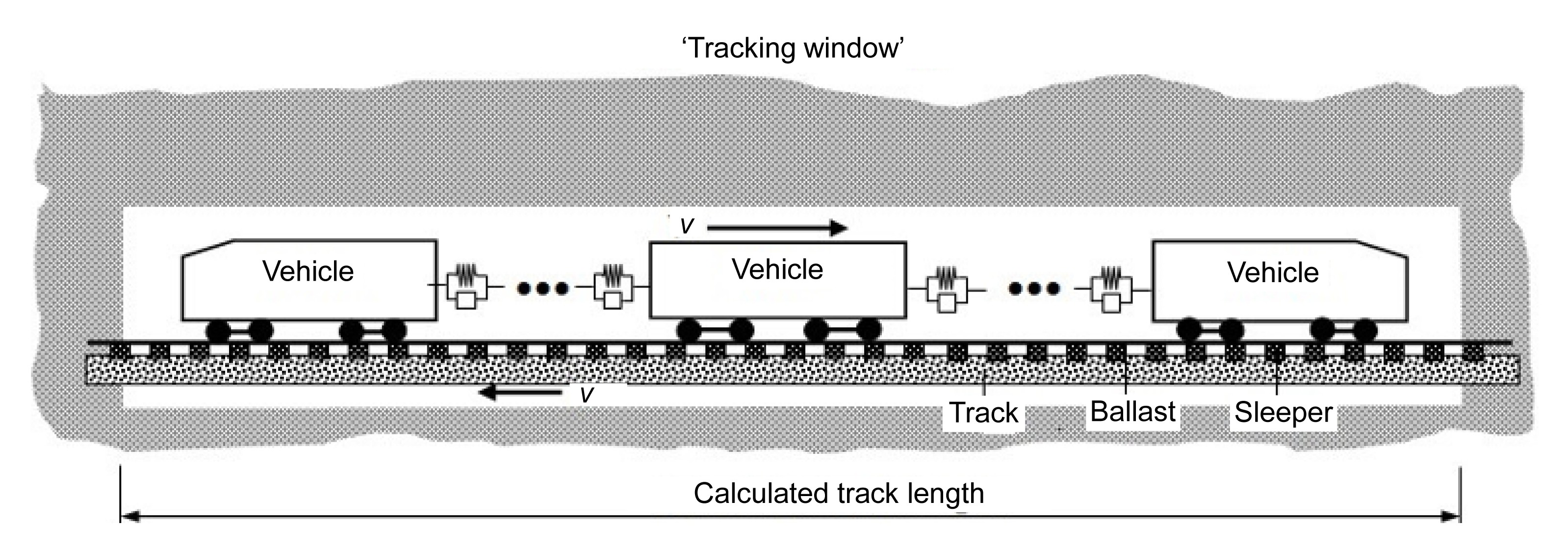
In the train/track dynamics calculation, there are four existing models (Popp et al., 1999): (1) the stationary load model; (2) the moving load model; (3) the moving irregularity model; and (4) the moving mass model. The most realistic one is the so-called moving mass model. However, it is very difficult to carry out numerical implementation using such a model because of the continuously updated track under the running train. For simplicity, a moving track support model (Xiao et al., 2007) developed by the authors is used to simulate the effect of the discrete periodic track support between the interaction of a high-speed vehicle and a track when high-speed trains run at constant speeds. The model of a half vehicle (one bogie) coupled with a track was extended to consider a whole vehicle (two bogies) in (Xiao et al., 2011). In this study, the model of Xiao et al. (2011) is further extended to consider the multi-vehicles of a train or the whole train coupled with a track, as shown in Fig. 8.
The model is seen as if one watches the behavior of a vehicle of the train running along the track through a window of ltim width. The window moves forward at the speed of the moving train. It is assumed that the vehicle always vibrates in the window. The track passes through the window in the inverse direction at the speed of the train, as shown in Fig. 8. The advantage of this model is that it allows rapid calculation of the train/track interaction of a train running on an infinitely long flexible track.
2.6. Initial and boundary conditions of the coupled train/track system
Before solving the equations of the dynamic system, the initial and boundary conditions should be prescribed. Both ends of the Timoshenko beam modeling the rails are hinged, and the deflections and the bending moments at the hinged beam ends are assumed to be zero. The vertical motion of the ballast bodies at both ends of the calculation track is assumed to be always zero, and the static state of the systems is regarded as the original point of reference. The initial displacements and velocities of all components of the track are set to zero. The initial displacements and the initial vertical and lateral velocities of all components of the high-speed train are also set to zero, and the initial longitudinal velocity is the running speed of the train, which is a constant.
It is obvious that the equations of coupled train/track model form a large-scaled nonlinear system. The stability, calculation speed, and accuracy of the numerical method for the equations are very important. A numerical method developed by Zhai (1996), termed as “new fast numerical integration for dynamics analysis of large systems”, is used to analyze the equations in a time step of 1.4×10⁻⁵ s in this study.
3. Verification of the train/track model
Based on the mathematical model described in Section 2, a computer simulation program, named high-speed train/track system dynamics (HSTTSD), was developed to analyze the dynamics of the coupled train/track system. To verify the 3D coupled train/track model, the dynamic results calculated by the present model are compared with those obtained by the commercial software SIMPACK. In this section, the vehicle/track dynamic interactions in the vertical and lateral directions are analyzed, by comparing the system responses obtained through HSTTSD and SIMPACK, under the excitation of vertical and lateral track irregularity on the tangent track. In the calculation, the vehicle parameters and the fastening parameters used are the same, and the vehicle speed is 300 km/h. The track irregularities are artificially generated sine-wave defects with a length of 20 m and an amplitude of 10 mm.
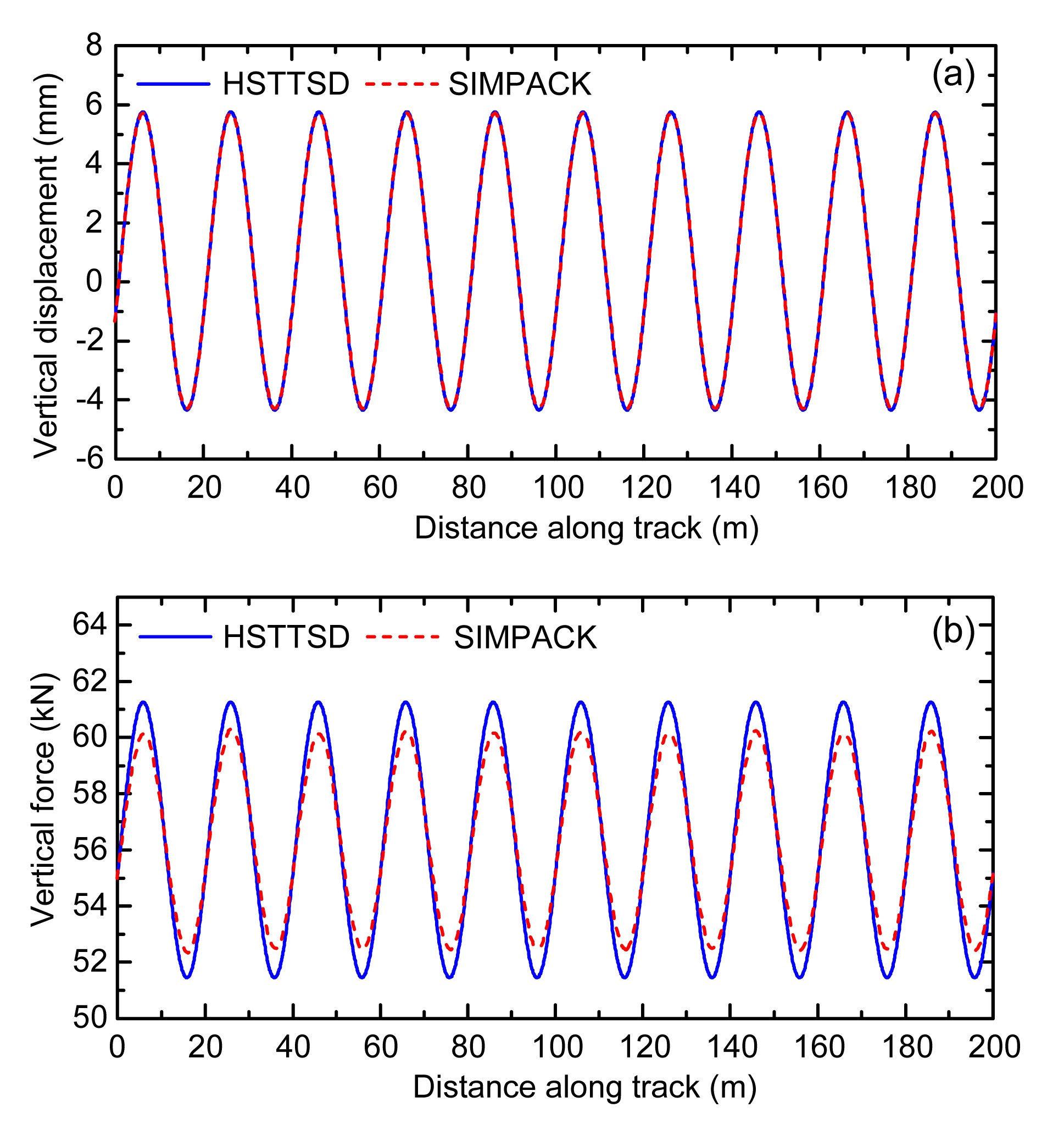
Figs. 9a and 9b are the wheelset vertical displacements and wheel/rail vertical forces, respectively, calculated by SIMPACK and HSTTSD. From Fig. 9, it is clear that the vertical displacements of the wheelsets are very close. Strictly speaking, the vertical displacement calculated by HSTTSD is a little larger than that obtained by SIMPACK, which is not clearly shown in Fig. 9a. The vertical force calculated by HSTTSD is also a little larger than that calculated by SIMPACK.
Fig.9 Comparison of vertical dynamic responses (a) Wheelset vertical displacement; (b) Wheel/rail vertical force
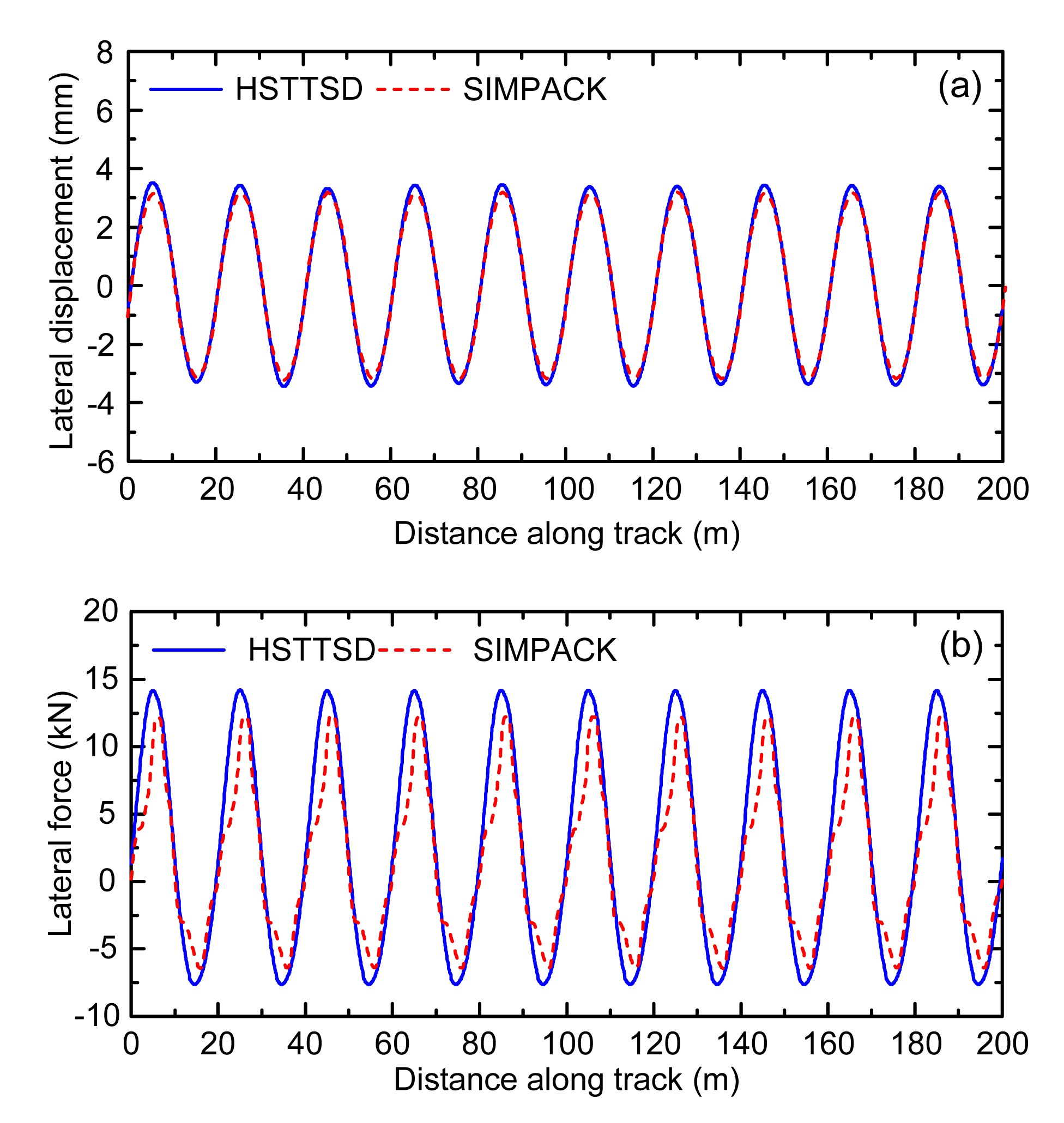
The lateral interaction of the wheel/rail system has a great influence on running safety against derailment of a train, and wear of the wheels and rails. Figs. 10a and 10b indicate the wheelset lateral displacements and wheel/rail lateral forces, respectively, achieved by SIMPACK and HSTTSD. It is obvious that the lateral displacements and forces calculated by HSTTSD are larger than those obtained by SIMPACK, which is similar to the phenomena that occurred in the results relating to the vertical interaction of the vehicle and the track, as described in Fig. 9.
Fig.10 Comparison of lateral dynamic responses (a) Wheelset lateral displacement; (b) Wheel/rail lateral force
The reason for the above phenomenon is that the track model in HSTTSD is different from that in SIMPACK. The track model in HSTTSD considers a flexible three-layer infrastructure consisting of rails, sleepers, and ballast bed. The connections between rails and sleepers, between sleepers and ballast blocks, and between ballast blocks and roadbed are replaced with the equivalent dampers and springs. The structure deformations of rails and sleepers are taken into account. Thus, the vertical (lateral) stiffness of the track characterized by HSTTSD is lower than that characterized by SIMPACK, which leads to the vertical (lateral) displacement calculated by HSTTSD being slightly larger than that obtained by SIMPACK, as shown in Figs. 9a and 10a.
Figs. 9b and 10b show that the difference between wheel/rail forces calculated by HSTTSD and by SIMPACK is significant, i.e., the relative errors are approximately 10%. Compared to the simplified track model in SIMPACK, the flexible track model in HSTTSD also considers the longitudinal propagating vibration waves induced in the rails and the periodical excitation caused by discrete sleepers. The structure deformation of rails, wave reflection from the adjacent wheels, and the moving track excitation may result in larger wheel/rail contact forces, and their corresponding contribution onto these differences needs to be examined in future work. However, the differences between the calculated results by the two models can be accepted in practice. Through the results discussed above, the proposed vehicle/track model is verified to be reliable, and it can be extended to a 3D coupled train/track model, as discussed in Section 2.
Through the comparisons, it can be concluded that the track model in HSTTSD is more reasonable than that of SIMPACK, because HSTTSD considers the flexibility and the dynamic behavior of the track components. But when we simulated a high-speed vehicle running over a 1000 m-length straight track at a speed of 350 km/h by using the Windows operating system on a 2.79 GHz CPU DELL Studio XPS (which has one node with eight processors), the computational time required for HSTTSD and SIMPACK was 470 s and 121 s, respectively. This means the computation speed for SIMPACK is approximately three times faster than that for HSTTSD. In other words, we should try to optimize the numerical algorithm to improve the calculation efficiency of the current model in the future.
4. Comparison of dynamic performances obtained by TTM and VTM
Traditional dynamics studies of railway vehicle/track systems were mainly based on the coupled VTM, while the cross-influence between the adjacent vehicles and the effect of the vehicle location in a train were neglected. However, the interaction of the neighboring vehicles has a great influence on the dynamic performance of the train/track system due to the tight-lock inter-vehicle connections installed on modern high-speed trains. In this situation, the difference in dynamic performance obtained by TTM and VTM should be taken into account. To obtain more accurate and reliable results from the dynamics simulation, the differences between the two types of dynamic models should first be pointed out.
In this section, several key dynamic performances, including vibration frequency response, ride comfort, and curving performance, obtained by TTM and VTM are compared, which will be discussed in Sections 4.1, 4.2, and 4.3. In the calculation, the TTM used a Chinese high-speed train comprised of eight vehicles coupled with the ballast track. For simplicity, the parameters of the vehicle and the track used in the two dynamic models are the same. The measured track irregularities of a Chinese high-speed line from Beijing to Tianjin were used in this calculation.
4.1. Comparison of vibration frequency components
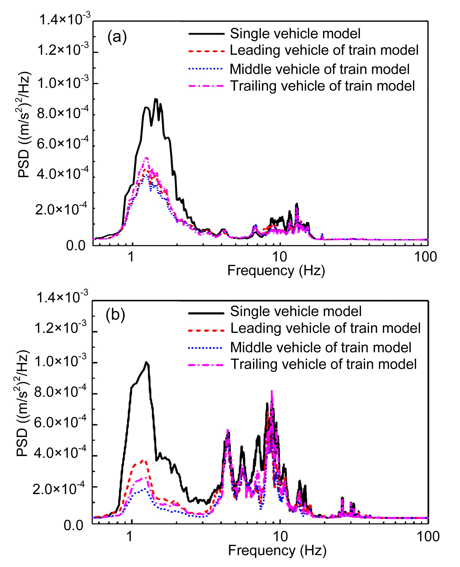
To make clear the differences in the dynamic performances obtained by TTM and VTM, the random responses of the car bodies, and the wheel/rail forces were firstly compared. In this simulation, the 3D high-speed train/track model described in Section 2 was used, a tangent track was considered, and the operating speed was 350 km/h. The power spectral densities (PSDs) of the vertical and lateral car body accelerations calculated by VTM and TTM are shown in Fig. 11, and the PSDs of the vertical and lateral wheel/rail forces are shown in Fig. 12. In these figures, the leading and trailing vehicles mean the 1st and 8th vehicles of the train, respectively, and the 4th vehicle is taken as the middle vehicle.
Fig.11 Comparison of car body vibration frequency components: (a) car body vertical acceleration PSD; (b) car body lateral acceleration PSD
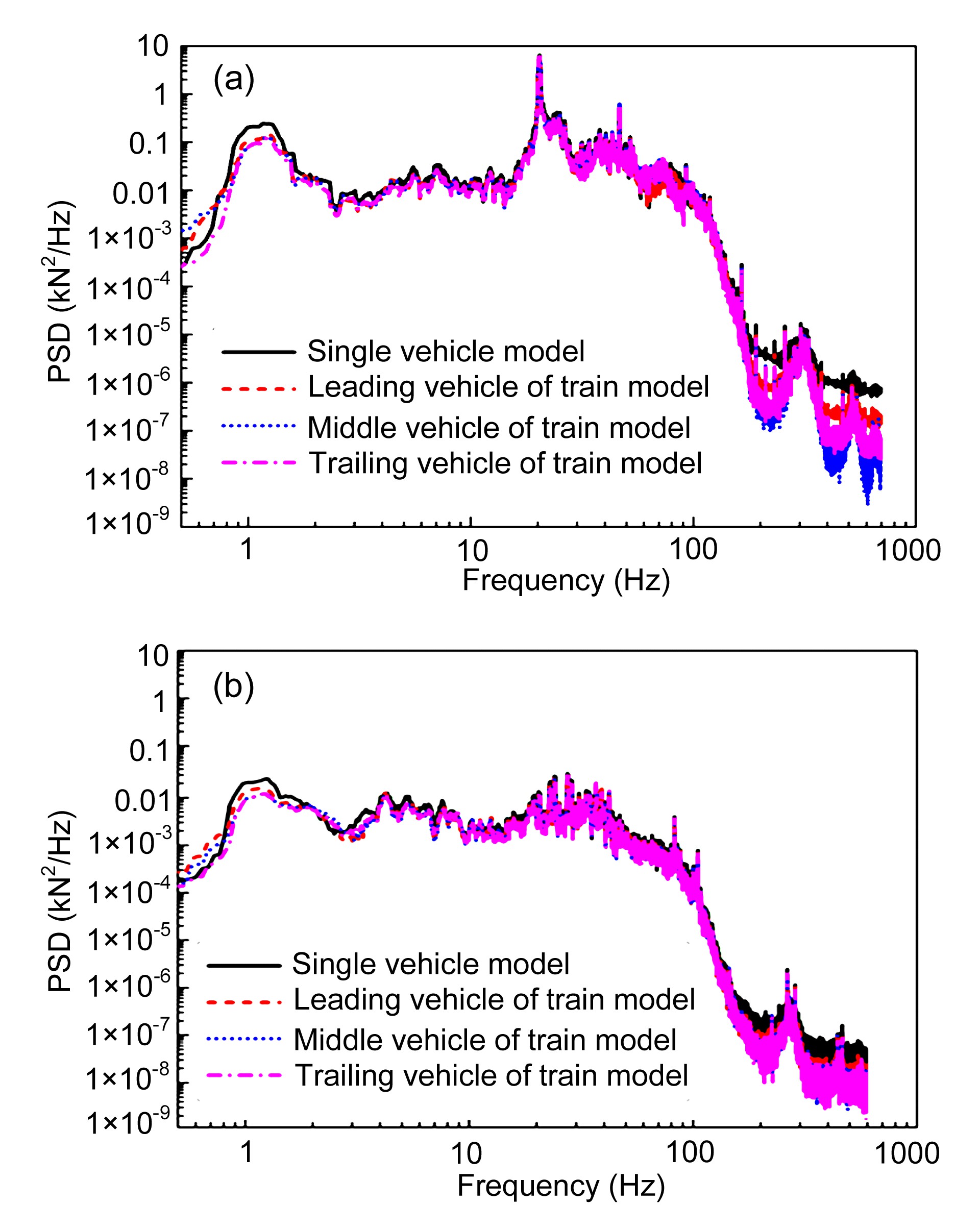
Fig.12 Comparison of wheel/rail force vibration frequency components: (a) wheel/rail vertical force PSD; (b) wheel/rail lateral force PSD
Fig. 11 shows significant difference occurs on vertical accelerations of the car body center upper the bogie for frequencies below 3 Hz, while 4 Hz for lateral accelerations, calculated by the two types of dynamic models, whereas the difference is small at higher frequencies due to the dominant low frequency vibration of the rigid car body model. From Fig. 11, it can be found that the car body PSD responses obtained by VTM are much higher than those obtained by TTM, especially in the frequency range of 1 Hz to 3 Hz. The reason for this phenomenon is that the tight-lock inter-vehicle connections between the adjacent vehicles of the train effectively restrain the relative motion of the neighboring vehicle ends, including the vertical, lateral, pitching, and yawing motions of the vehicles. The role of the tight-lock inter-vehicle connections can be characterized in TTM. But in VTM, the two ends of the car body are considered to be free. In this situation, the motions at the ends of the vehicle calculated by VTM are larger than those calculated by TTM, especially at low frequencies. From Fig. 11, it can also be seen that the PSD of the middle car is lower than those of the leading car and trailing car, especially at 1–3 Hz, as shown in Fig. 11b. For vertical car body acceleration, the peak response quite often occurs in the trailing car, while the greatest lateral acceleration of the car body is found in the leading car.
Fig. 12 indicates the PSDs of the vertical and lateral wheel/rail forces of the first left wheel achieved by VTM and TTM. From Fig. 12, it can be seen that there is a little difference between the wheel/rail vertical and lateral forces calculated by the two models in the frequency range below 100 Hz, but there is a significant difference at higher frequencies. The wheel/rail force PSD obtained from VTM is larger than that obtained from TTM in the high frequency range. These differences are caused by the wave reflections between the wheels. Wu and Thompson (2002) pointed out that there is a big difference between the wheel/rail contact forces in the frequency region of 550–1200 Hz obtained by a multiple-wheel/rail interaction model and a single-wheel/rail interaction model due to the effect of wave reflections between the wheels.
This explanation is also appropriate for the results of Fig. 12. The first wheelset of VTM receives wave reflections from three other wheelsets, while the leading wheelset of TTM receives reflections from 31 other wheelsets. These wave reflections between wheels would make the responses of wheel/rail interaction calculated by VTM and TTM different. The wheel/rail force PSD of the leading car is larger than those of the middle car and trailing car in the frequency range of more than 100 Hz. The vertical wheel/rail PSD of the middle car is the smallest, compared to those of the leading and trailing cars.
The comparison shown in Figs. 11 and 12 clearly indicates that there is a significant difference in the dynamic behavior characteristics of the vehicles characterized by VTM and TTM. The vehicle location also has an important influence on the dynamic behavior. It is important to consider the vehicle location and the cross-influence of adjacent vehicles in the analysis of vertical and lateral car body accelerations in the frequency range below 20 Hz and the wheel/rail force variations at high frequencies.
4.2. Comparison of ride comfort
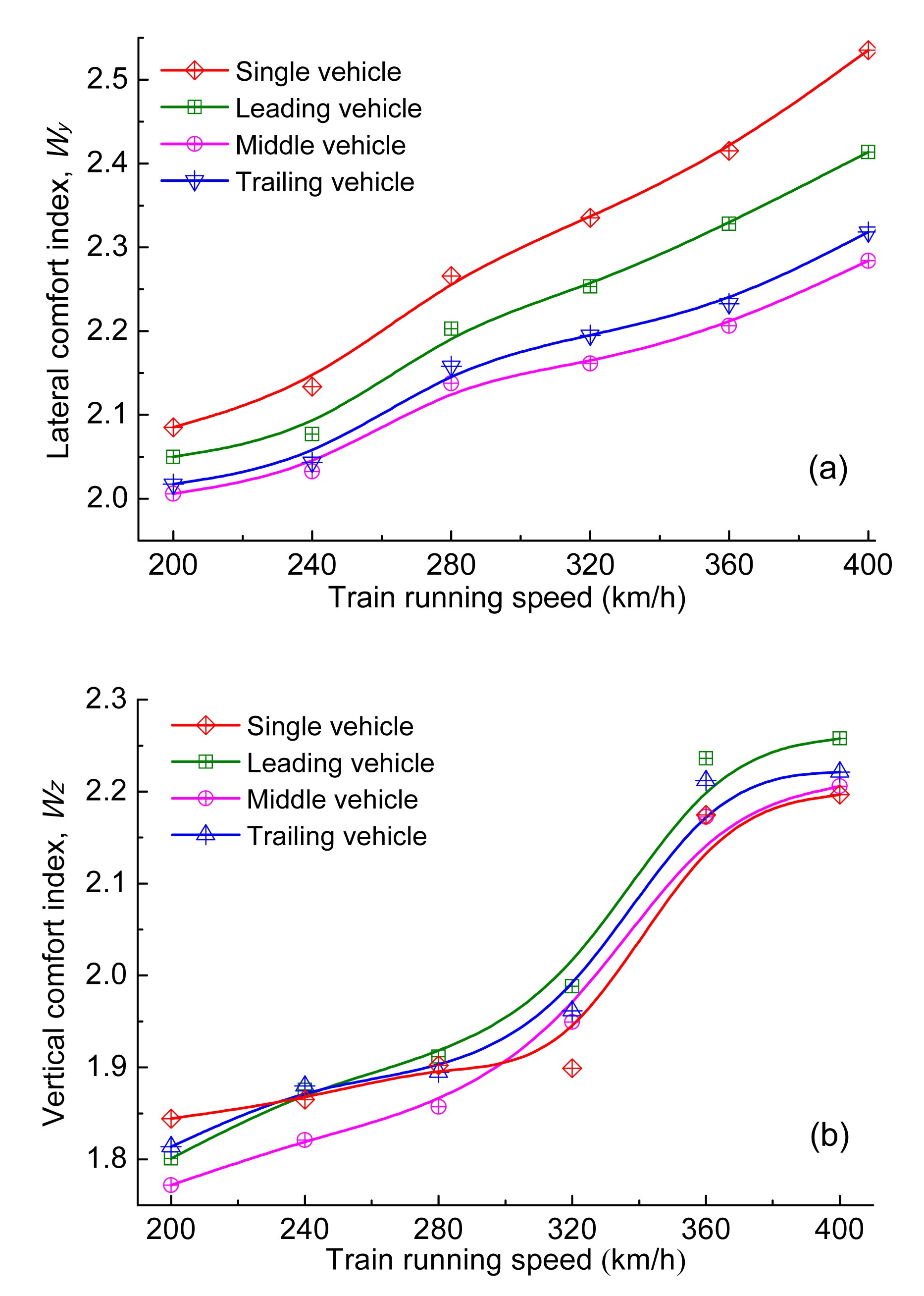
The ride comfort, one of the key dynamic performance targets of high-speed trains, is closely related to the vibration characteristics of the car body in the low frequency range. The analysis in Section 4.1 indicates that the vibration frequency components of the car body in the frequency range below 20 Hz obtained by VTM and TTM are very different, which means the ride comforts calculated by the two types of dynamic models are different. To clarify this difference, a comparison of ride comfort performance is carried out in this section. In this calculation, the tangent ballast track was used, and the operating speed ranged from 200 to 400 km/h. Other parameters were the same as those used in Section 4.1. The comparison results of the lateral and vertical Sperling comfort indexes are shown in Fig. 13.
Fig.13 Comparison of ride comfort: (a) lateral Sperling comfort index; (b) vertical Sperling comfort index
From Fig. 13a, it can be clearly seen that the lateral Sperling comfort index calculated by VTM is larger than that calculated by TTM in all speed ranges. The maximum difference in the results between the single vehicle model and the middle vehicle and the leading vehicle reach 0.25 and 0.11, respectively. The difference between the two types of dynamic models increases with increasing train speed. When the running speed reaches 400 km/h, the maximum lateral Sperling comfort indexes of the leading vehicle, middle vehicle, and the trailing vehicle, calculated by TTM, are 2.42, 2.28, and 2.32, respectively. However, the maximum lateral Sperling comfort index of VTM reaches 2.53, which is greater than the comfort index limit value of the ‘Excellent grade’ used in Chinese Railways (SAC, 1985). It means that the lateral comfort of high-speed trains would be overestimated by VTM in practical engineering application. Thus, when the lateral comfort of high-speed trains is investigated though numerical simulation, using TTM is more reasonable. The vehicle location also has a great influence on the ride comfort. Among the three vehicles compared, the lateral comfort index of the middle car is the smallest in the speed range, and the ride comfort of the leading car is the worst.
Compared to the obvious difference of the lateral comfort indexes calculated by the two models, the difference of the vertical comfort indexes is not so significant, as shown in Fig. 13b. From the comparison results of the vertical comfort index, it can be concluded that VTM is appropriate for analyzing the vertical comfort index of the vehicles when a long high-speed train operates on a tangent track without serious irregularities, such as corrugated rails, rail welding dips, and track subsidence. However, it can be expected that if the track irregularity is severe, the difference of the vertical ride comfort when using these two models would be large. Furthermore, the operating speed has a great influence on the ride comfort. With increasing speed, the differences in the lateral and vertical Sperling comfort indexes calculated by the two models increase rapidly.
4.3. Comparison of curving performance
When a high-speed train negotiates a curved track, large lateral forces are generated between the wheels and rails. These large lateral forces, in combination with the small vertical forces, may cause wheel climbing and rail rollover as the train negotiates the curve. Therefore, curving performance is very important for evaluating the running safety of high-speed trains. In this section, the curving performances obtained by TTM and VTM are compared. The curved track had a circle curve radius of 9000 m, a transition curve length of 490 m, a circle curve length of 400 m, and a super elevation of 125 mm. The running speed of the train ranged from 200 to 400 km/h. The track irregularities and other concerned parameters are the same as in Section 4.1.
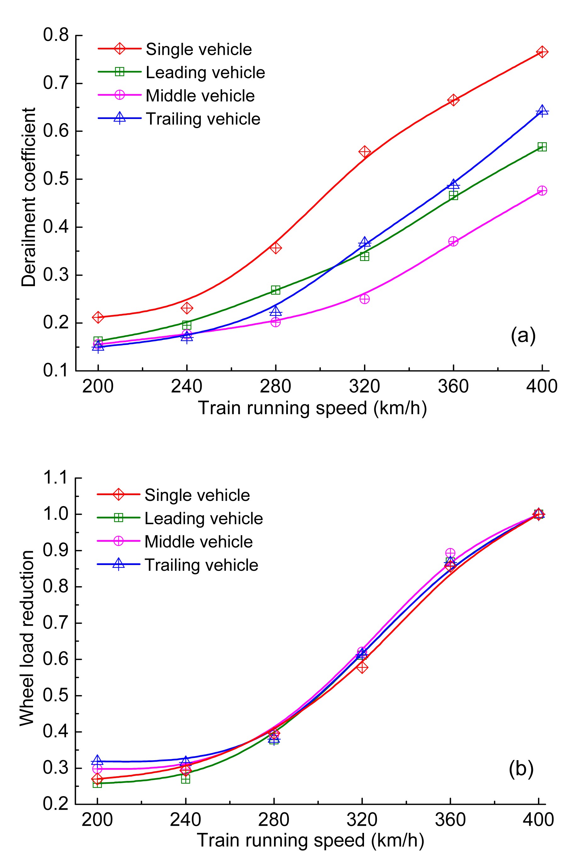
To evaluate curving performance, two safety criteria used in Chinese Railway were selected. One is the derailment coefficient (or Nadal coefficient) (SAC, 1985) defined as the ratio of the lateral force to the total vertical force on the same wheel. The other is the wheel load reduction, which is defined as the ratio of the reduction in the vertical dynamical forces on both wheels of a wheelset to the total vertical wheelset loading. The total vertical force is the sum of the static wheel load and the dynamic vertical force on the same wheel. The safety limit values of both derailment coefficient and wheel load reduction are 0.8 in the evaluation of the operating safety of high-speed trains in China. TTM and VTM are used to calculate the two safety criteria when the train passes over curved track at different speeds. The calculated results are compared and discussed as follows.
Fig. 14 shows the maximum values of the dynamic derailment coefficient and wheel loading reduction of all the wheelsets calculated by VTM and TTM. As expected, the derailment coefficient and wheel loading reduction increase as the train speed increases. When the train speed is greater than 350 km/h, the maximum wheel loading reduction is greater than its safety limit value, 0.8. This means that the running speed of the high-speed train should be limited when it is negotiating a curved track.
Fig.14 Comparison of dynamic performances on a large radius curved track: (a) derailment coefficient; (b) wheel load reduction
From Fig. 14, it can also be seen that the interaction of neighboring vehicles and the vehicle location have a large effect on the derailment coefficient, but their effects on wheel unloading are not significant due to the large radius of the curved track. Fig. 14a illustrates the great difference of derailment coefficients calculated by the two models. The derailment coefficient calculated by VTM is much larger than those calculated by TTM in all the analyzed speed ranges. Specifically, the derailment coefficient calculated using VTM is larger than reality when the train passes over the curved track. The maximum difference occurs between the single vehicle model and the middle vehicle, which are calculated by VTM and TTM, respectively. Compared to the results of the leading and trailing vehicles of the same train, the derailment coefficient of the middle vehicle is the smallest. Note that the difference of the results obtained with the two models increases with increasing operating speed. On the other hand, Fig. 14b shows a good agreement between the wheel load reductions calculated by the two models in all the analyzed speed ranges under the present curved track conditions. However, it can be predicted that if the radius of the curved track is small, the difference of wheel load reductions calculated by the two models would be large.
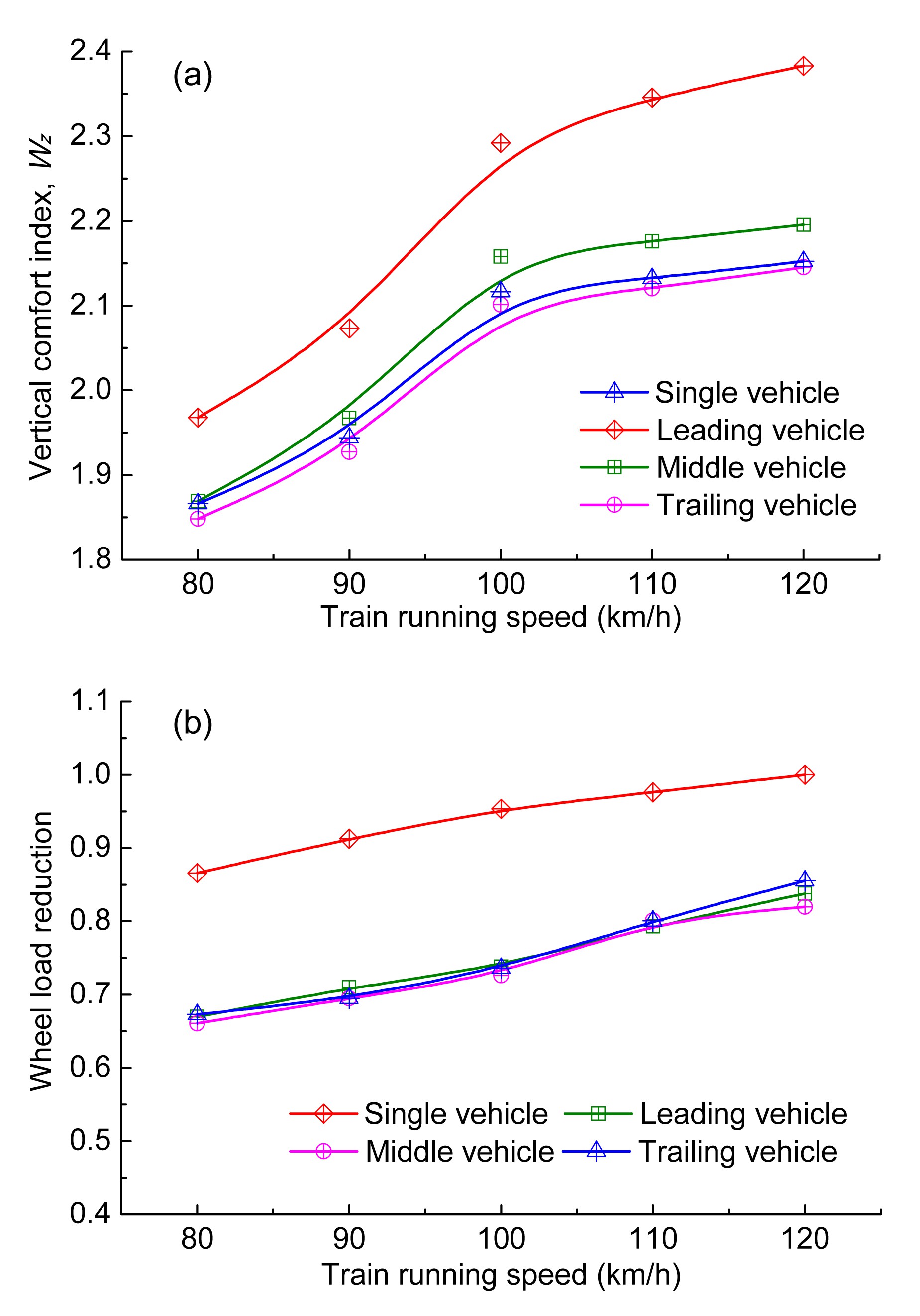
The above results discussed show that the vertical comfort indexes on the tangent track and the wheel load reduction on large radius curved tracks calculated by VTM and TTM are close. However, if the operating ambient is bad or the radius of the curved track is small, how much would be the difference between the two types of dynamic models? To measure that difference, a comparison of the dynamic responses on a small radius curved track obtained by TTM and VTM is carried out. The curved track has a circle curve radius of 600 m, a transition curve length of 100 m, a circle curve length of 280 m, and a cant of 100 mm. The operating speed of the train ranges from 80 to 120 km/h and other concerned parameters used in this numerical simulation are the same as in Section 4.1. Fig. 15 shows the results of vertical comfort indexes and wheel load reductions calculated by VTM and TTM, respectively.
Fig.15 Comparison of dynamic performance on a small radius curve track: (a) vertical Sperling comfort indexes; (b) wheel load reductions
The difference in the dynamical behavior calculated by the two models is evident for a train operating on a curved track with a relatively small radius. The dynamical behavior of the different vehicles of the same train calculated by TTM is also different under the same operating conditions. From Fig. 15a, the differences of vertical comfort indexes of these vehicles increase with increasing operating speed. Fig. 15b shows that the wheelset load reductions of the vehicles approach to 1 with increasing operating speed. This is because the speed increase causes the normal load between the wheels and the low rail reduce to zero, that is to say, the wheels lose contact with the low rail.
Through the detailed comparisons of the results obtained by VTM and TTM, it is noticeable that the dynamical behavior of the vehicle/track system calculated by VTM will be overstated, and it is more reasonable that TTM is used to calculate the dynamic behavior of the train and the track, especially in the situation of trains with strong lateral and vertical vibrations. Since the neighboring vehicles of a train influence each other and each vehicle has different boundary conditions, the dynamic behavior of each vehicle is different from the others in the same train. Therefore, it is necessary that a 3D dynamic model of a train coupled with a flexible track is carried forward to estimate the dynamical behavior of the train and the track in high-speed operations.
5. Conclusions
A 3D dynamic model of a nonlinear high-speed train coupled with a flexible ballast track is put forward. The advantages of this model are: (1) the mutual influence of the adjacent vehicles on the dynamic behavior of high-speed vehicles and the track is considered; (2) it is possible to carry out fast dynamics calculations on a long train running on an infinitely long flexible track. The reliability of the 3D coupled train/track model was verified through a detailed numerical comparison with the commercial software SIMPACK, and the difference caused by the track modeling was then analyzed. Several key dynamic performances, including vibration frequency components, ride comfort, and curving behavior, obtained by TTM and VTM, are compared and discussed. Subsequently, the following conclusions were reached:
There is a distinct difference in the vibration frequency components calculated between VTM and TTM. The inter-vehicle connections of a train have an important influence on the dynamic behavior of a car body in the frequency range below 20 Hz and the wheel/rail forces at high frequencies.
The lateral comfort index calculated by VTM is greater than that calculated by TTM, which can be predicted. Therefore, in practical engineering applications, using TTM is more reasonable. The vertical comfort indexes obtained by the two models are close when the train operates on a curved track of large radius, but the difference is very large when the train operates on a small radius curved track.
The difference of derailment coefficients obtained by the two models is very large when the train negotiates curved tracks with large radii. It is obvious that the derailment coefficient is overestimated using VTM, and using TTM is more reasonable in practical engineering applications. The wheel load reductions obtained by the two models have a good agreement when the train operates on a curved track with a large radius. If the radius of the curved track is small, the difference is obvious.
The difference in lateral dynamic behavior is relatively large when looking at different vehicle locations in a high-speed train, but the difference in vertical dynamic performance is relatively small when a high-speed train operates on a usually tangent track. Among the vehicles of a long train, the results calculated by TTM show that the ride comfort and curving performance of the intermediate vehicles are better than those of the leading and trailing vehicles because the two ends of the intermediate vehicles are restrained by their neighbors.
[1] Arnold, M., Burgermeister, B., Fhrer, C., 2011. Numerical methods in vehicle system dynamics: state of the art and current developments. Vehicle System Dynamics, 49(7):1159-1207.
[2] Baeza, L., Ouyang, H., 2011. A railway track dynamics model based on modal substructuring and a cyclic boundary condition. Journal of Sound and Vibration, 330(1):75-86.
[3] Cai, Y., Sun, H., Xu, C., 2008. Response of railway track system on poroelastic half-space soil medium subjected to a moving train load. International Journal of Solids and Structures, 45(18-19):5015-5034.
[4] Chen, G., Zhai, W.M., 2004. A new wheel/rail spatially dynamic coupling model and its verification. Vehicle System Dynamics, 41(4):301-322.
[5] Di Gialleonardo, E., Braghin, F., Bruni, S., 2012. The influence of track modelling options on the simulation of rail vehicle dynamics. Journal of Sound and Vibration, 331(19):4246-4258.
[6] Evans, J., Berg, M., 2009. Challenges in simulation of rail vehicle dynamics. Vehicle System Dynamics, 47(8):1023-1048.
[7] Frhling, R.D., 1998. Low frequency dynamic vehicle/track interaction: modelling and simulation. Vehicle System Dynamics, 29(S1):30-46.
[9] Jin, X.S., Wu, P.B., Wen, Z.F., 2002. Effects of structure elastic deformations of wheelset and track on creep forces of wheel/rail in rolling contact. Wear, 253(1-2):247-256.
[10] Jin, X.S., Wen, Z.F., Zhang, W.H., 2005. Numerical simulation of rail corrugation on curved track. Computers and Structures, 83(25-26):2052-2065.
[11] Jin, X.S., Wen, Z.F., Wang, K.W., 2006. Three-dimensional train-track model for study of rail corrugation. Journal of Sound and Vibration, 293(3-5):830-855.
[12] Jin, X.S., Xiao, X.B., Ling, L., 2013. Study on safety boundary for high-speed trains running in severe environments. International Journal of Rail Transportation, 1(1-2):87-108.
[13] Ju, S.H., Li, H.C., 2011. Dynamic interaction analysis of trains moving on embankments during earthquakes. Journal of Sound and Vibration, 330(22):5322-5332.
[14] Kalker, J.J., 1967. On the Rolling Contact of Two Elastic Bodies in the Presence of Dry Friction. PhD Thesis, Delft University,the Netherlands :
[15] Knothe, K., Grassie, S.L., 1993. Modeling of railway track and vehicle/track interaction at high frequencies. Vehicle System Dynamics, 22(3-4):209-262.
[16] Lei, X.Y., Mao, L.J., 2004. Dynamic response analyses of vehicle and track coupled system on track transition of conventional high speed railway. Journal of Sound and Vibration, 271(3-5):1133-1146.
[17] Nielsen, J.C., Igeland, A., 1995. Vertical dynamic interaction between train and track-influence of wheel and track imperfections. Journal of Sound and Vibration, 187(5):825-839.
[18] Oscarsson, J., Dahlberg, T., 1998. Dynamic train/track/ballast interaction—computer models and full-scale experiments. Vehicle System Dynamics, 29(S1):73-84.
[19] Popp, K., Kruse, H., Kaiser, I., 1999. Vehicle-track dynamics in the mid-frequency range. Vehicle System Dynamics, 31(5-6):423-464.
[20] SAC (Standardization Administration of the Peoples Republic of China), 1985. Railway vehiclesSpecification for evaluation the dynamic performance and accreditation test, GB/T 5599-85. (in Chinese), SAC,China :
[21] Shen, Z.Y., Hedrick, J.K., Elkins, J.A., 1983. A comparison of alternative creep-force models for rail vehicle dynamic analysis. Vehicle System Dynamics, 12(1-3):79-83.
[22] Sun, Y.Q., Dhanasekar, M., 2002. A dynamic model for the vertical interaction of the rail track and wagon system. International Journal of Solids and Structures, 39(5):1337-1359.
[23] Sun, Y.Q., Dhanasekar, M., Roach, D., 2003. A three-dimensional model for the lateral and vertical dynamics of wagon-track systems. Proceedings of the Institution of Mechanical Engineers, Part F: Journal of Rail and Rapid Transit, 217(1):31-45.
[24] Tanabe, M., Matsumoto, N., Wakui, H., 2008. A simple and efficient numerical method for dynamic interaction analysis of a high-speed train and railway structure during an earthquake. Journal of Computational and Nonlinear Dynamics, 3(4):041002
[25] Wang, K., 1984. The track of wheel contact points and the calculation of wheel/rail geometric contact parameters. Journal of Southwest Jiaotong University, (in Chinese),19(1):88-99.
[26] Wu, T.X., Thompson, D.J., 2002. Behaviour of the normal contact force under multiple wheel/rail interaction. Vehicle System Dynamics, 37(3):157-174.
[27] Xia, H., Zhang, N., Roeck, G.D., 2003. Dynamic analysis of high-speed railway bridge under articulated trains. Computers and Structures, 81(26-27):2467-2478.
[28] Xiao, X.B., Jin, X.S., Wen, Z.F., 2007. Effect of disabled fastening systems and ballast on vehicle derailment. Journal of Vibration and Acoustics, 129(2):217-229.
[29] Xiao, X.B., Jin, X.S., Wen, Z.F., 2011. Effect of tangent track buckle on vehicle derailment. Multibody System Dynamics, 25(1):1-41.
[30] Xiao, X.B., Ling, L., Jin, X.S., 2012. A study of the derailment mechanism of a high speed train due to an earthquake. Vehicle System Dynamics, 50(3):449-470.
[31] Xiao, X.B., Ling, L., Xiong, J.Y., 2014. Study on the safety of operating high-speed railway vehicles subjected to crosswinds. Journal of Zhejiang University-SCIENCE A (Applied Physics & Engineering), 15(9):694-710.
[32] Yang, Y.B., Wu, Y.S., 2002. Dynamic stability of trains moving over bridges shaken by earthquakes. Journal of Sound and Vibration, 258(1):65-94.
[33] Zhai, W.M., 1996. Two simple fast integration methods for large-scale dynamic problems in engineering. International Journal for Numerical Methods in Engineering, 39(24):4199-4214.
[34] Zhai, W.M., Cai, C.B., Guo, S.Z., 1996. Coupling model of vertical and lateral vehicle/track interactions. Vehicle System Dynamics, 26(1):61-79.
[35] Zhai, W.M., Wang, K.Y., Cai, C.B., 2009. Fundamentals of vehicle-track coupled dynamics. Vehicle System Dynamics, 47(11):1349-1376.
[36] Zhang, S.G., 2009. Design Method of High-speed Train. (in Chinese), Chinese Railway Press,Beijing, China :
[37] Zhou, L., Shen, Z.Y., 2013. Dynamic analysis of a high-speed train operating on a curved track with failed fasteners. Journal of Zhejiang University-SCIENCE A (Applied Physics & Engineering), 14(6):447-458.
Open peer comments: Debate/Discuss/Question/Opinion


 ORCID:
Open peer comments: Debate/Discuss/Question/Opinion
<1>