Affiliation(s):
1.
Institute of Cryogenics and Refrigeration, Zhejiang University, Hangzhou 310027, China; moreAffiliation(s): 1.
Institute of Cryogenics and Refrigeration, Zhejiang University, Hangzhou 310027, China; 2.
School of Information and Electrical Engineering, Zhejiang University City College, Hangzhou 310015, China; 3.
Shanghai Institute of Technical Physics, Chinese Academy of Sciences, Shanghai 200083, China; less
Zhi-hua Gan, Long-yi Wang, Sheng-ying Zhao, Yu-jing Song, Wei-wei Wang, Yi-nong Wu. Acoustic impedance characteristics of linear compressors[J]. Journal of Zhejiang University Science A, 2013, 14(7): 494-503.
@article{title="Acoustic impedance characteristics of linear compressors", author="Zhi-hua Gan, Long-yi Wang, Sheng-ying Zhao, Yu-jing Song, Wei-wei Wang, Yi-nong Wu", journal="Journal of Zhejiang University Science A", volume="14", number="7", pages="494-503", year="2013", publisher="Zhejiang University Press & Springer", doi="10.1631/jzus.A1300113" }
%0 Journal Article %T Acoustic impedance characteristics of linear compressors %A Zhi-hua Gan %A Long-yi Wang %A Sheng-ying Zhao %A Yu-jing Song %A Wei-wei Wang %A Yi-nong Wu %J Journal of Zhejiang University SCIENCE A %V 14 %N 7 %P 494-503 %@ 1673-565X %D 2013 %I Zhejiang University Press & Springer %DOI 10.1631/jzus.A1300113
TY - JOUR T1 - Acoustic impedance characteristics of linear compressors A1 - Zhi-hua Gan A1 - Long-yi Wang A1 - Sheng-ying Zhao A1 - Yu-jing Song A1 - Wei-wei Wang A1 - Yi-nong Wu J0 - Journal of Zhejiang University Science A VL - 14 IS - 7 SP - 494 EP - 503 %@ 1673-565X Y1 - 2013 PB - Zhejiang University Press & Springer ER - DOI - 10.1631/jzus.A1300113
Abstract: The acoustic field of a linear compressor serves to deliver the compression work to the load, such as the connected cold head of a cryocooler; it plays an equivalently important role as the electrical and mechanical parts, especially in the impedance match issue. This paper studies the acoustic impedance characteristics of a linear compressor. The parameters including the current, the piston displacement, the pressure amplitude, the electrical power dissipation, the power factor, the pressure-volumetric (PV) power delivered, and the efficiency are theoretically and experimentally investigated. Different from previous theoretical studies, optimization for the operations away from the resonance is also included. More general optimization results imply relevance between thermoacoustic engines and linear compressors. The predicted results are validated by the experiments performed on a linear compressor with an adjustable resistive-capacitive (RC) acoustic load. The comparisons between the calculations and the measurements are presented and analyzed. The results provide deeper insight into the mechanism of the linear compressor and the impedance match in a cryocooler system.
Darkslateblue:Affiliate; Royal Blue:Author; Turquoise:Article
Article Content
1. Introduction
The linear compressor possesses the advantages of oil-free, high reliability, low vibration, and long-life operation. Since being introduced for the first time in 1981 (Davey, 1981), they are often used to drive cryocoolers to ensure long-life and high-reliability (Nast et al., 2006; Raab and Tward, 2010). The operation of the linear compressor comprises complex transition processes among the electrical, mechanical, and acoustic fields.
Previous studies reported the dynamic characteristics of linear compressors. However, the acoustic impedance on the piston was modeled using a simple equivalent damping coefficient and a gas spring stiffness (Koh et al., 2002; Park et al., 2002; Chen et al., 2007; Chen and Zhu, 2012). For the application in cryogenic fields, the acoustic field is equivalently important because it delivers the compression power to the load, which is usually a connected cold head (Radebaugh et al., 2010). The impedance match between them is a key to optimizing the system performance. Therefore, quantitative calculations of the acoustic characteristics and their coupling with the electric and mechanical fields are fundamental.
Wakeland (2000) used an equivalent circuit model to analyze the performance and optimized the acoustic resistance Ra under the resonant condition. He found that the optimum efficiency of a linear compressor can be obtained when Ra=σRm/A2, where σ is a compressor constant, Rm is the mechanical resistance, and A is the piston area. Swift (2002) also derived the efficiency using acoustic impedance analyses, and optimized the piston area A at resonance. Radebaugh et al. (2010) discussed the acoustic impedance match based on a given commercial linear compressor. Dai et al. (2011) analyzed the impedance matching principle between the linear compressor and the cold head from the perspective of an energy balance. However, most of the work mentioned above were focused on the resonant operation, which in practice is difficult to achieve. For example, the impedance of a cold head is often optimally designed such that the volume flow rate leads the pressure wave by tens of degrees at the hot end, that is at the piston (Gan et al., 2008), which does not always fit the best output characteristics of a given compressor, hence non-resonance usually occurs. Also, the effects of acoustic impedance on the parameters, except for pressure-volumetric (PV) power and efficiency, remain unanswered. Bao et al. (2006) studied the effect of a resistive-capacitive (RC) load on the performance of a thermoacoustic system and investigated a wide range of acoustic impedance. It was experimentally found that a maximum PV power or efficiency can be obtained when the acoustic resistance equals the acoustic reactance. However, this is different from the conclusion of Wakeland (2000) and not always valid for a linear compressor (Gan et al., 2012; Wang et al., 2012).
This paper focuses on developing a general expression for the dependence of performance on a variety of related parameters, including the current, the piston displacement, the pressure amplitude, the electrical power dissipation, and the power factor. The PV power delivered and the efficiency of a linear compressor are optimized without the assumption that the compressor and the load are in a resonant status. The effects of acoustic impedance on the output characteristics of the compressor are discussed. Experiments are carried out using the RC load approach to validate the calculations.
2. Theoretical analysis
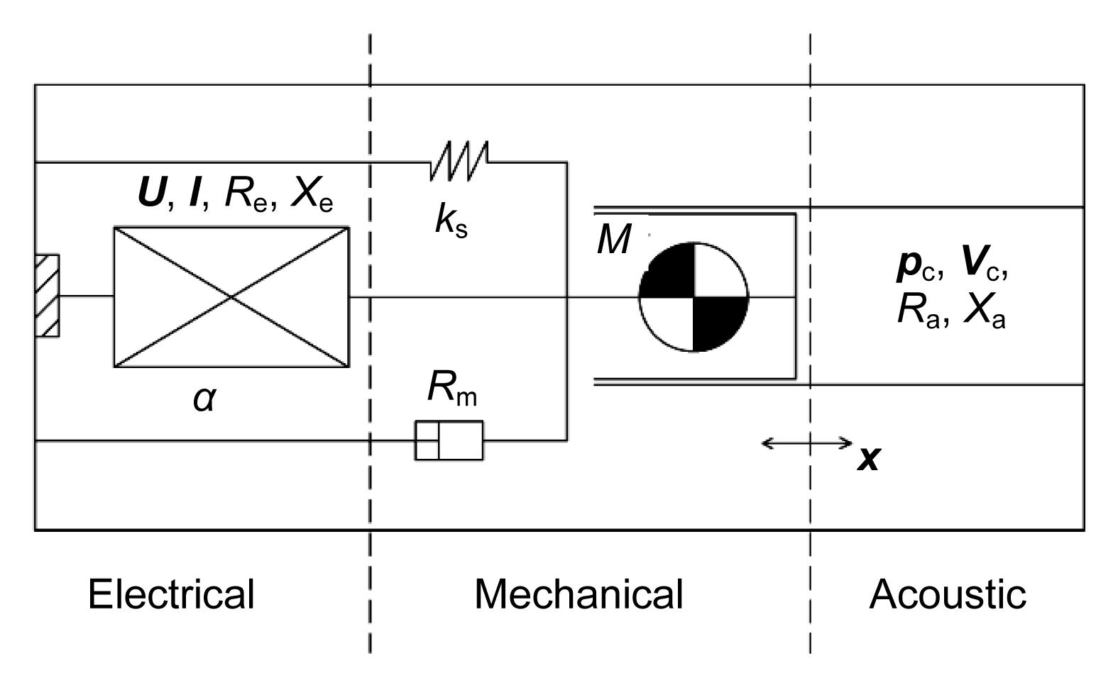
The linear compressor shown in Fig. 1 is a kind of electrodynamic device, which can be described by the following linear harmonic-approximation equations (Swift, 2002):
, ,
where U is the complex voltage across the electric terminals, the bold font representing the complex vectors, Re is the electric resistance, I is the complex electric current, Le is the electric inductance, α is the transduction coefficient which is the product of the magnetic field and the length of the wire in the field, Vc is the volume flow rate at the piston face, pc is the pressure amplitude inside the compression volume, j equals ,
M is the moving mass, ω=2πf is the angular frequency, and ks is the mechanical spring stiffness. These two equations express Ohm’s law and Newton’s law, respectively. Here, the electrical impedance Ze, the mechanical impedance Zm, and the acoustic impedance on the piston Za are defined as
, , ,
where Ra is the acoustic resistance, Xe, Xm, and Xa express the electrical, mechanical and acoustic reactance, respectively. By solving Eqs. (1)−(5), we derive the expressions of I, piston displacement x, and pc as follows:
, , .
Fig.1 Physical model of a linear compressor
Then the input electrical power can be obtained:
.
The PV power on the piston is expressed as
.
Hence, the ratio of Eqs. (9) and (10) gives the efficiency of the transformation of electric to PV power on the piston:
.
Eq. (11) is equivalent to that in (Wakeland, 2000; Swift, 2002) but is derived in a straightforward way. It is found that Xe is absent in Eq. (11), which means that the electrical inductance has no influence on η although it affects the We and WPV terms.
An equivalent mechanical reactance X combining the mechanical and acoustic impedances is defined as (Wakeland, 2000)
.
Note that X here has the essential meaning because when X=0, the system is known to be at resonance. In a similar way, an equivalent mechanical resistance R combining the mechanical and acoustic impedances is defined as
.
Substituting Eqs. (12) and (13) into Eqs. (9) and (11), respectively, leads to simple and accessible forms:
, .
A total impedance is defined as
.
The first term of Eq. (16), in other words the real part of Z, represents the equivalent electrical resistance, while the second term, in other words the imaginary part of Z, represents the equivalent electrical reactance. Since the power can be only dissipated in the real part of the impedance, the PV power efficiency can be also obtained from the fractional contribution of the acoustic resistance to the total equivalent resistance from Eq. (16), hence, the same result as Eq. (15) can be obtained.
The power factor can be expressed as
.
Eq. (17) indicates that the power factor is not only related to the electrical part, but also to the mechanical as well as the acoustic domain. The highest power factor does not accompany the highest efficiency (X=0). In other words, when the power factor equals 1, it does not mean that the system is at resonance. A capacitor in series with the coil is necessary to shift the electrical resonance (cosθU-I=1) to the mechanical resonance (X=0) which allows Xe=0.
Differentiating Eq. (10) with respect to Ra and setting the result equal to zero gives the maximum PV power:
, .
Differentiating Eq. (11) with respect to Ra without the assumption of X=0, and equating the result to zero, we obtain the optimum of Ra as
,
where determines the highest possible efficiency of a linear compressor (Wakeland, 2000). For this value of Ra, the efficiency has its maximum value of
.
Eqs. (20) and (21) are obtained for the first time by the present authors without the resonance assumption. When the compressor is at resonance (X=0), Eqs. (20) and (21) are simplified to
.
Eq. (22) is the same as derived by Wakeland (2000) and Dai et al. (2011).
For a thermoacoustic system, there are no mechanical components, therefore Rm=Xm=0, and Eq. (20) simplifies to , which is the same as found by Bao et al. (2006). Although thermoacoustic engines are far more complicated than that described in Eqs. (1) and (2), the foregoing analyses without resonance assumption imply some relevance between thermoacoustic engines and linear compressors.
3. Experimental setup
To verify the analyses above and to investigate the effects of acoustic impedance on the performance of the linear compressor over a wide range of Ra, experimental studies are carried out. The experimental setup consists of a linear compressor with a swept volume of 3.6 cm3 and an RC load. The measured parameters of the linear compressor are listed in Table 1.
Table 1
Parameters of the linear compressor
Re (Ω)
Le (mH)
Rm (kg/s)
M (kg)
ks (N/m)
α (N/A)
A (m2)
2.3
1.66
0.6
0.13
5360
18.0
2.01×10⁻⁴
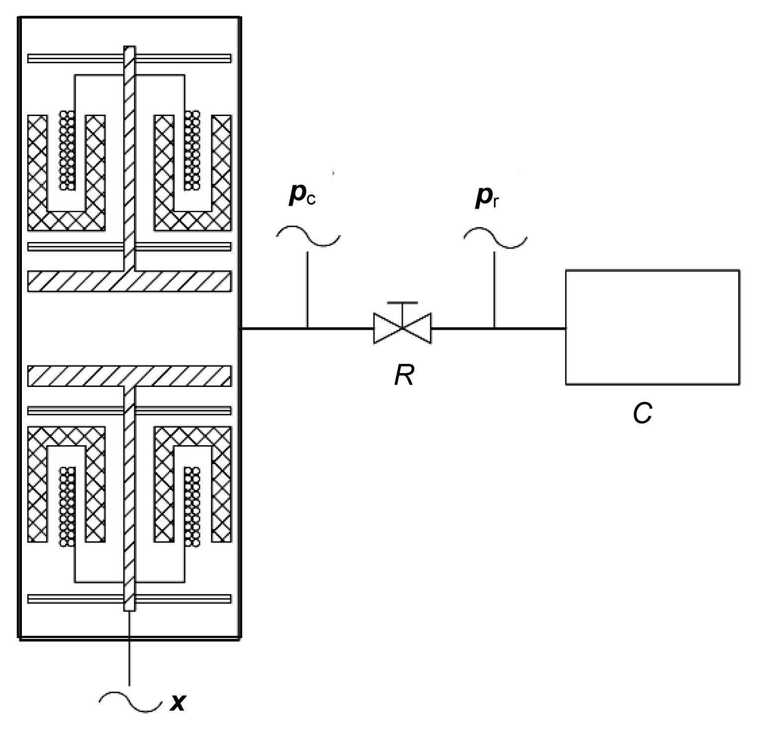
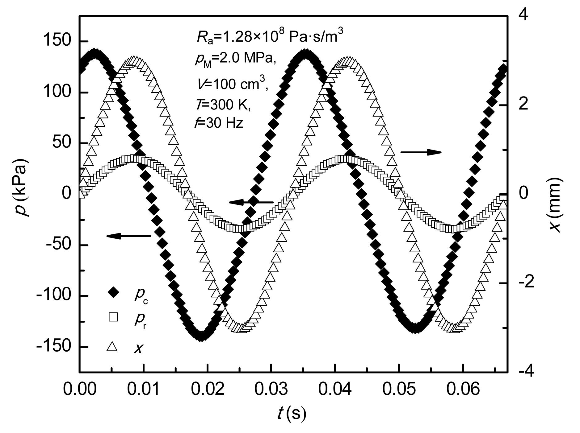
The RC load comprises a needle valve and a reservoir, as shown in Fig. 2. Helium gas was employed here. Two piezoelectric-type pressure transducers pc and pr are mounted before and after the valve in the experiments, respectively. The current, the power factor, and the electrical power are obtained from the power meter. A linear variable displacement transducer (LVDT) is mounted on one piston end of the compressor to measure the displacement. Fig. 3 shows the measured pressure and displacement waves, which are all sinusoidal. The delivered PV power can be calculated as
,
where is the phase difference between pc and x. When a linear compressor is operating, the PV power delivered to the RC load is dissipated in the valve (R). The compression volume is small enough to be ignored, and the reservoir is made of stainless steel which can be considered as an adiabatic reservoir; hence, Ra and Xa are equal to the resistance of the valve (R) and the capacitance of the reservoir (C), respectively, which are given by (Bao et al., 2006)
where is the phase difference between pc and pr, γ is the specific heat ratio of the working gas, pM is the mean charging pressure, and V is the volume of the reservoir.
Fig.2 Schematic of an RC load driven by a linear compressor
Fig.3 Measured waves of pressures and displacement
During the experiments, Ra is changed by regulating the valve openings, while Xa is changed by using various reservoir volumes and operating frequencies.
4. Analyses and discussion
4.1. Volume influence
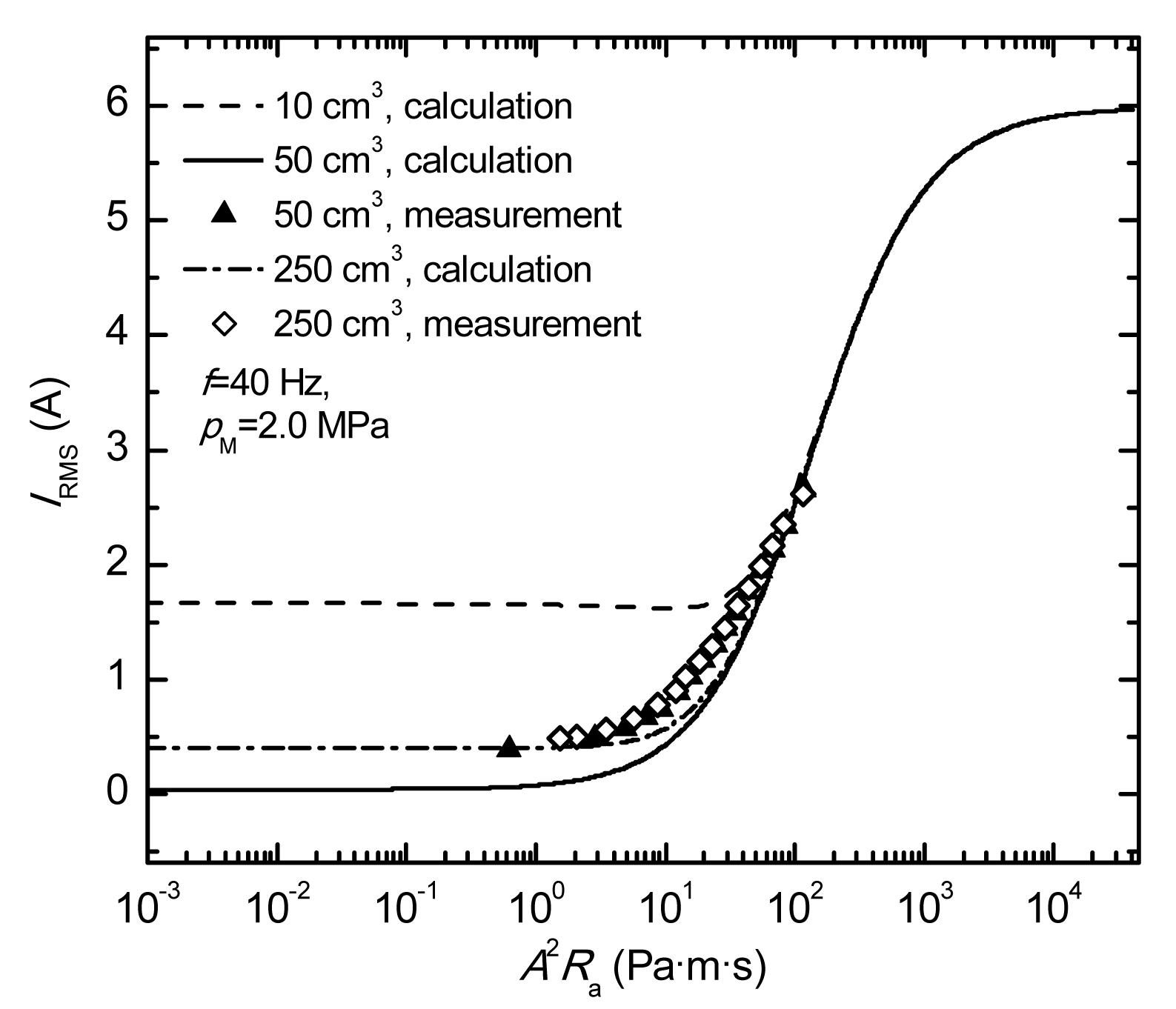
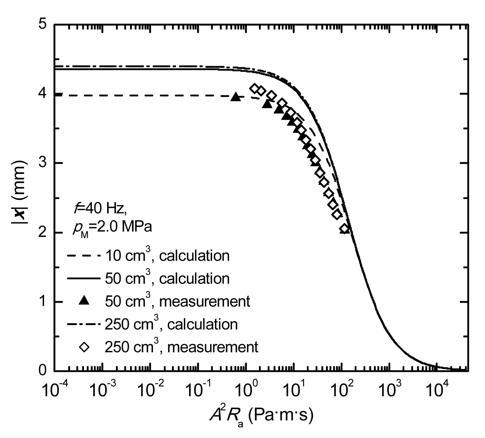
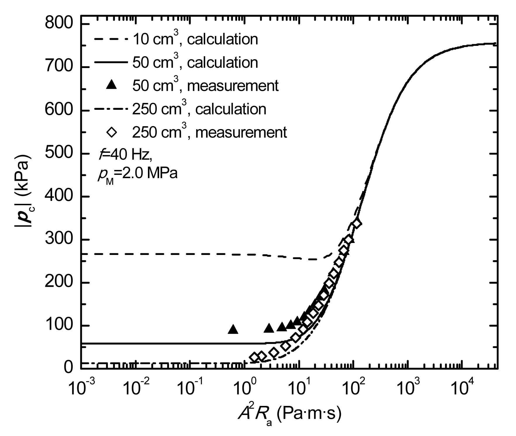
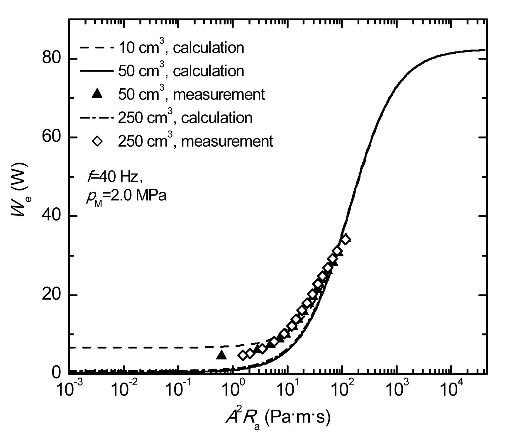
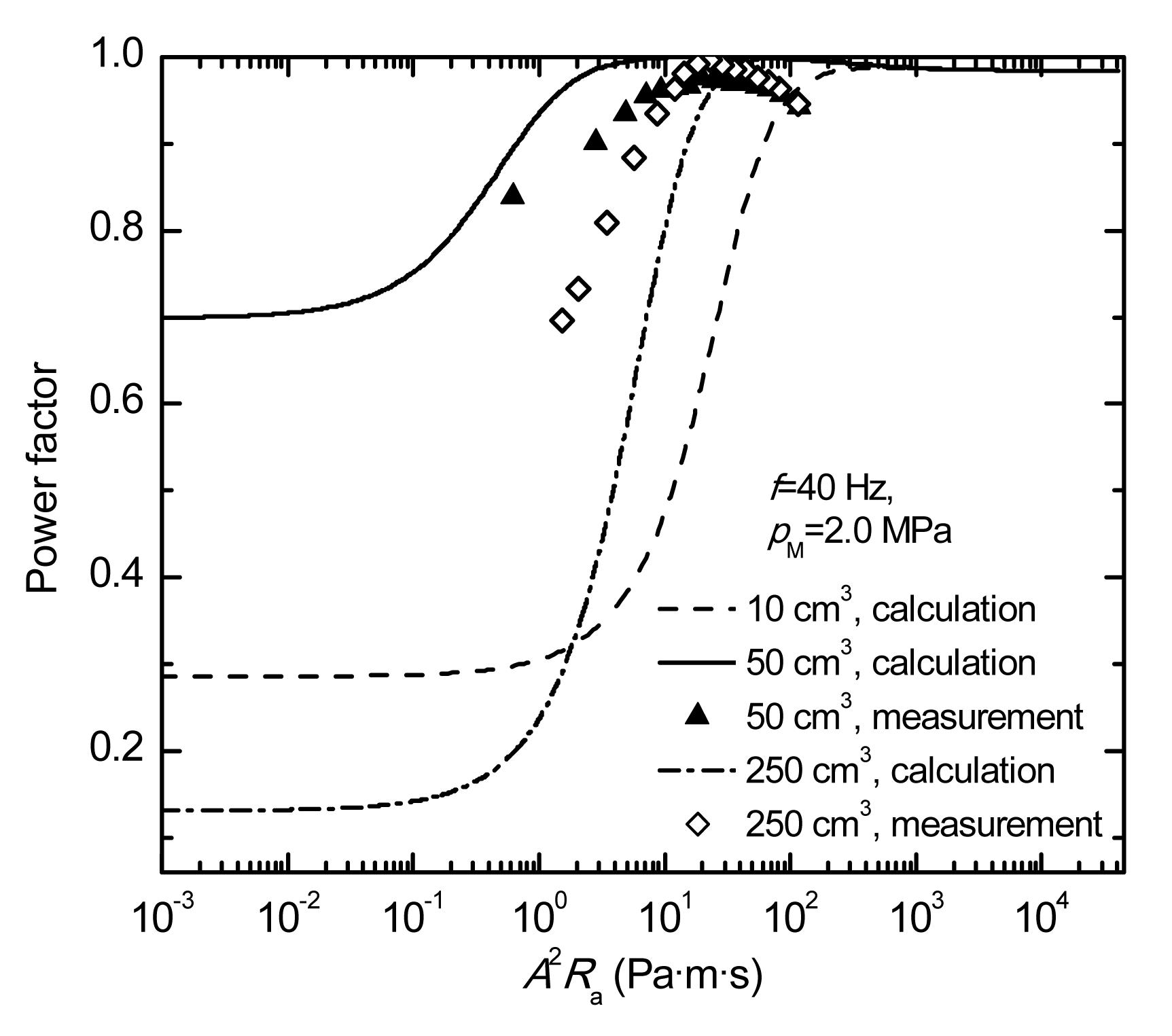
Figs. 4−10 compare the theoretical predictions of the root mean square (RMS) current IRMS, piston displacement amplitude |x|, pressure amplitude |pc|, electric power, power factor, PV power, and the efficiency with the corresponding experimental results with different volumes of the reservoir. In the calculations and experiments, the input RMS voltage URMS of the compressor is 14 V, the charging pressure in the system is 2.0 MPa, and f is 40 Hz. A2Ra is used as the abscissa instead of Ra because it has the same unit of Rm. The calculations are carried out in a wide range of A2Ra between 10−3–105 Pa·m·s, while the experiments are performed within the range of A2Ra between 100–102 Pa·m·s. Here, different volumes will only result in different values of Xa. On the whole, the model and experimental results agree well with each other.
Fig.4 RMS current vs. acoustic resistance under different volumes
Fig.5 Piston displacement amplitude vs. acoustic resistance under different volumes
Fig.6 Pressure amplitude at load inlet vs. acoustic resistance under different volumes
Fig.7 Electrical input power vs. acoustic resistance under different volumes
Fig.8 Power factor vs. acoustic resistance under different volumes
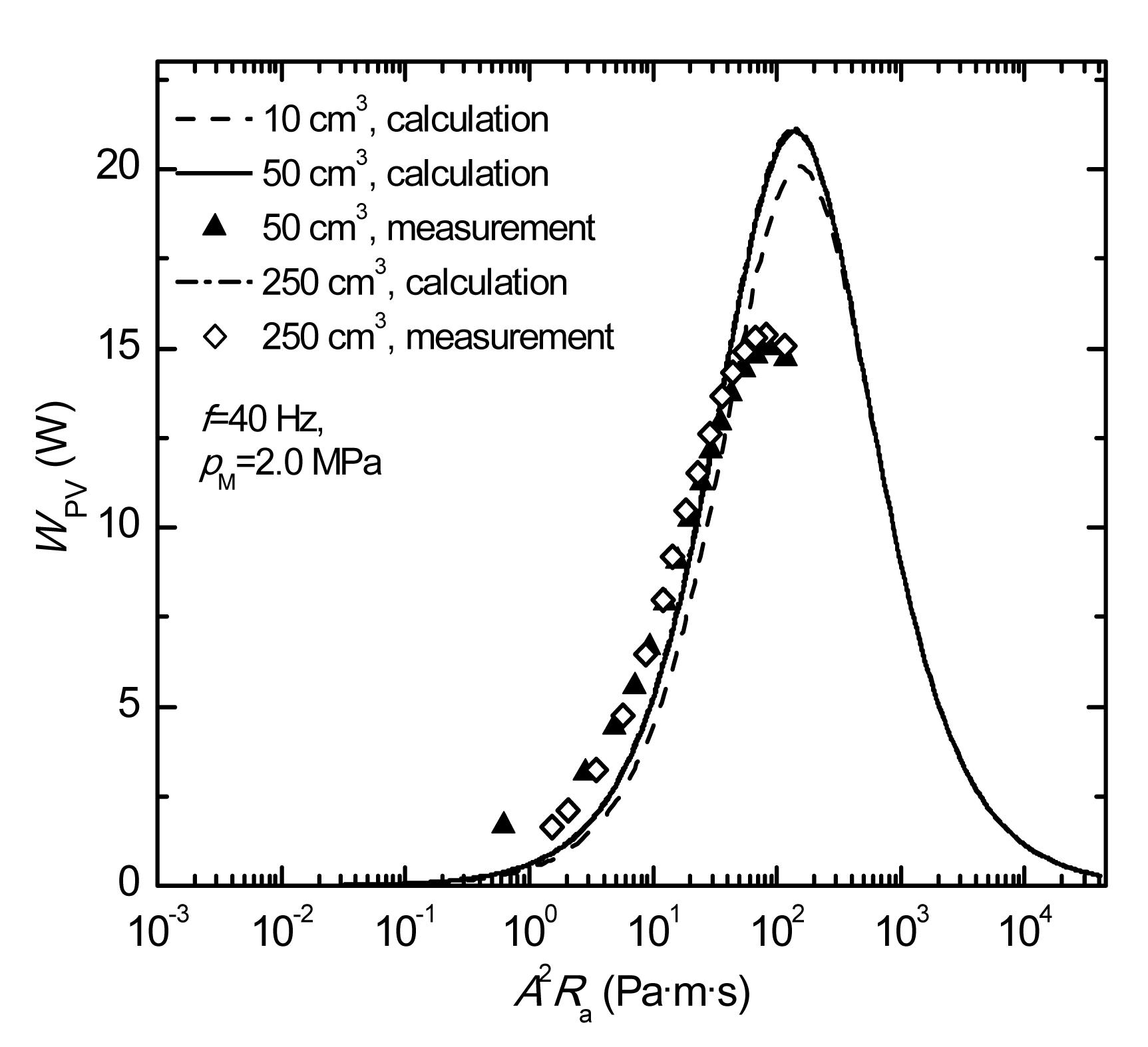
Fig.9 PV power delivered vs. acoustic resistance under different volumes
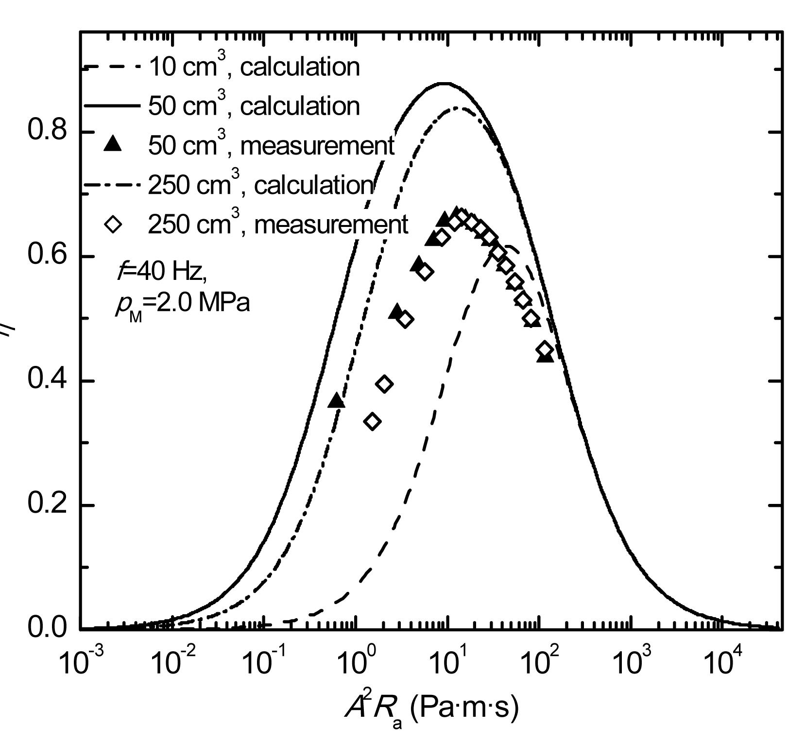
Fig.10 Efficiency vs. acoustic resistance under different volumes
The deviations between measurements and calculations are due to several aspects that are neglected in our calculations, for example the eddy current loss and the hysteresis loss inside the yokes (Reed et al., 2006), the blow-by through the clearance seal (Reed et al., 2006), the irreversible heat transfer inside the compression volume (Reed et al., 2004), and the pressure amplitude in the back volume. So the measured WPV is less than the calculations (Fig. 9), thus the efficiency is lower (Fig. 10). Moreover, the static electrical inductance employed here is different from the dynamic electrical inductance, which results in the deviation between measurements and calculations in Fig. 8.
It is shown in Figs. 4−10 that all these parameters (IRMS, |x|, |pc|, We, power factor, WPV, and η) are affected by A2Ra in a wide range (10−3−105 Pa·m·s), when Ra is much smaller than Xa, then Xa, or in other words V, is the decisive factor for the performance. When Ra is comparable with Xa, both Ra and Xa have an equivalent impact on the performance. When Ra is much larger than Xa, it determines the performance of the linear compressor.
Along with the increase of Ra, the magnitude |Z| of the total equivalent impedance Z, shown in Eq. (16), decreases; therefore IRMS and We increase for a given voltage. The equivalent damping coefficient R increases, hence, |x| decreases. Thus, as indicated by Eq. (2), more motor force is applied to the gas inside the compression volume, as a result, |pc| increases. In the range where |x| decreases (Fig. 5) and |pc| increases (Fig. 6), WPV exhibits a peak as shown in Fig. 9. As for the power factor, it reaches a peak value of 1 at the condition of , and it will finally reach the value when Ra becomes infinite. The variation of η can be explained from the tendencies of both WPV and We, or by examining the variation of the fractional contribution of the acoustic resistance to the total equivalent resistance as given by Eq. (16). As Ra goes up, this contribution first increases, peaks, and then decreases.
As the reservoir volume, V increases, |x| increases and |pc| decreases, IRMS and We decrease at first and then increase, while the power factor and η increase at first and then decrease. With this linear compressor, for the given conditions of 40 Hz and 2.0 MPa, we have Xm=11.4 kg/s, and A2Xa=−53.6, −10.7, and −2.15 Pa·m·s for V of 10 cm3, 50 cm3 and 250 cm3, respectively. Here, the volume of 50 cm3 provides the approximate resonant operation (X=0), and the efficiency η also reaches its maximum.
It is also interesting to note that the curves in Fig. 10 are symmetric about Ra on the logarithmic scale. A brief mathematical explanation of this feature is provided in the Appendix.
4.2. Frequency influence
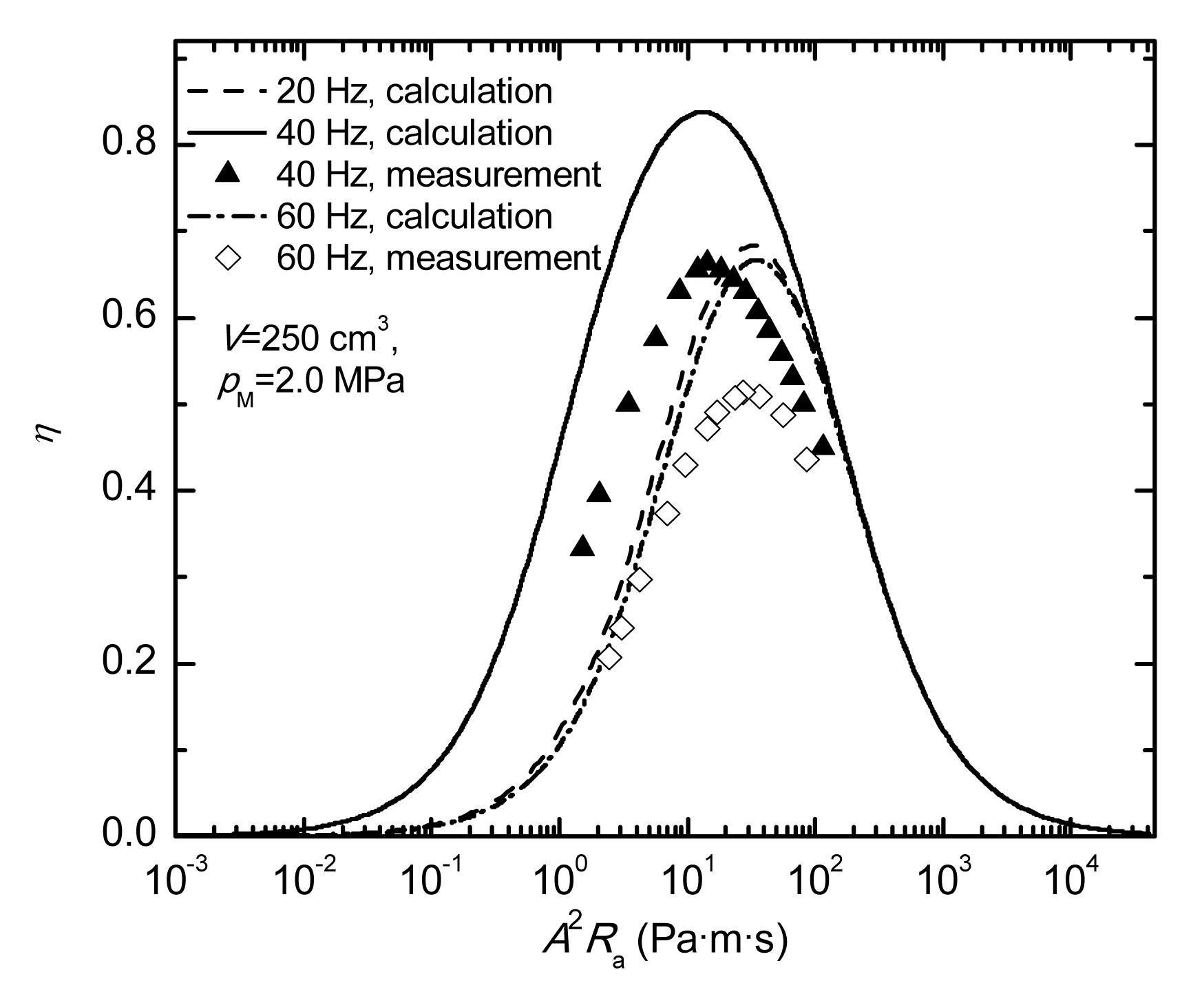
The effects of frequency on the compressor performance have also been investigated. Figs. 11–17 compare the theoretical predictions with the corresponding experimental results at different frequencies. Here, in the calculations and experiments, the input voltage URMS of the compressor is 11 V, the charging pressure in the system is 2.0 MPa, and V is 250 cm3. Unlike the effect of V, different values of f will result in not only different values of Xa, but also different values of Xe and Xm. Also, it is found that the tendencies in the theoretical results describe the experimental data.
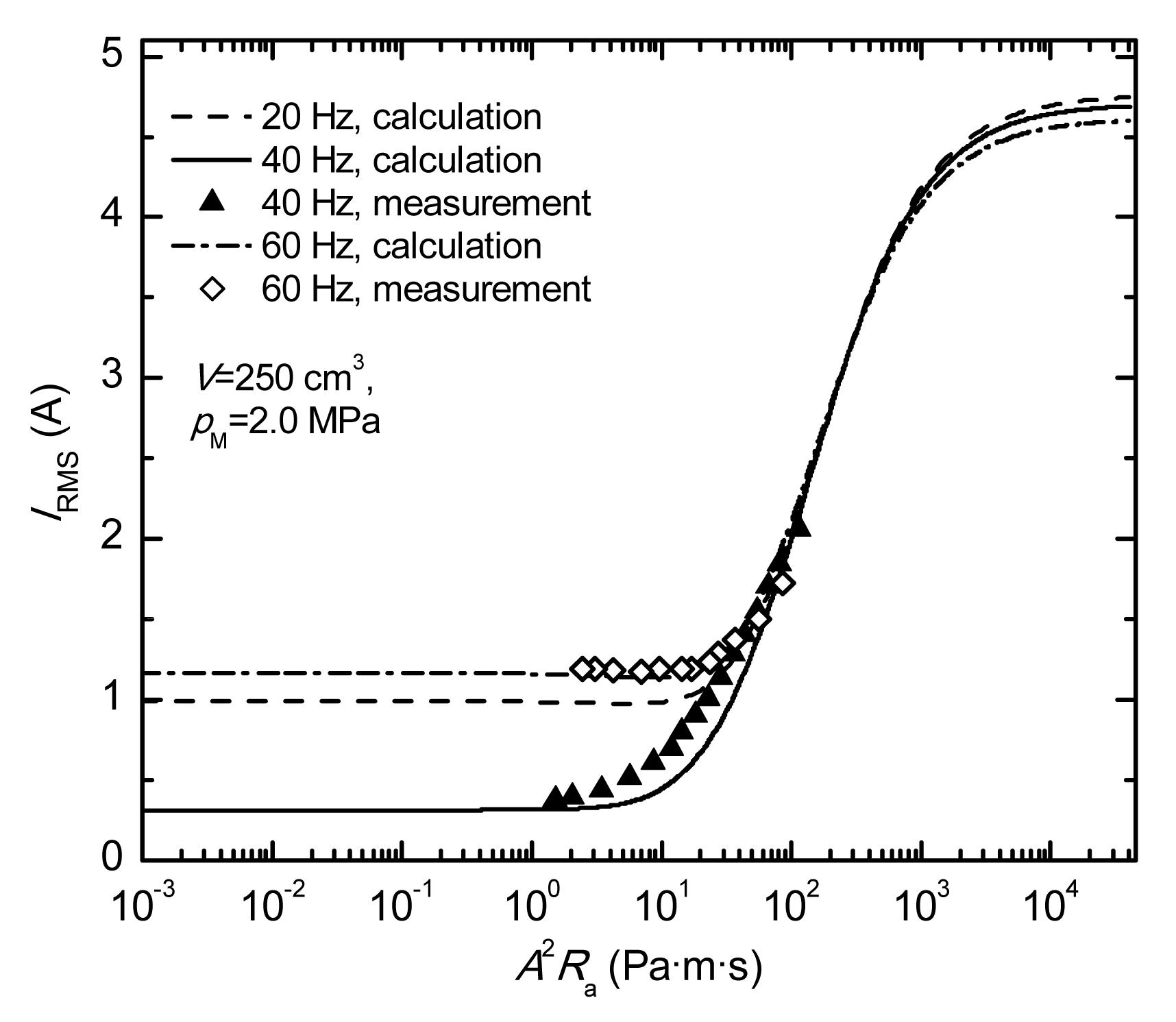
Fig.11 RMS current vs. acoustic resistance under different frequencies
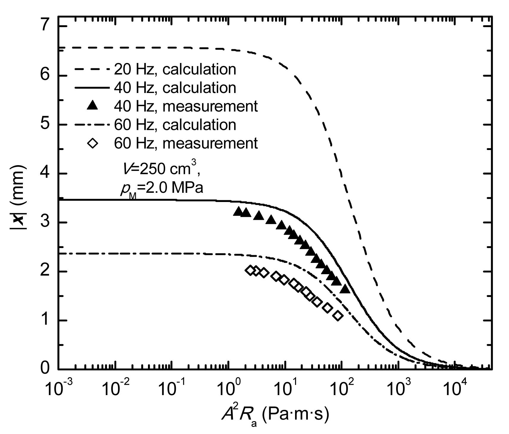
Fig.12 Piston displacement amplitude vs. acoustic resistance under different frequencies
Fig.13 Pressure amplitude at load inlet vs. acoustic resistance under different frequencies
Fig.14 Electrical input power vs. acoustic resistance under different frequencies
Fig.15 Power factor vs. acoustic resistance under different frequencies
Fig.16 PV power delivered vs. acoustic resistance under different frequencies
Fig.17 Efficiency vs. acoustic resistance under different frequencies
The effects of acoustic impedance at different frequencies f are similar to those at different reservoir volumes V. An exception occurs when Ra is much larger than Xa; in this range of Ra the performance is mainly determined not only by Ra but also by f (because f affects Xe and Xm). When Ra is much smaller than Xa, an increase in f results in a decrease in both |x| and |pc|, whereas IRMS and We decrease at first and then increase, and η increases at first and then decreases. Also, some losses, for example the eddy current loss and the hysteresis loss inside the yokes, increase with frequency increases, that is why the PV power of 60 Hz in Fig. 16 is smaller than that of 40 Hz at their peak values.
Eqs. (6), (8) and (9) indicate that when Ra becomes infinite, I, pc, and We will reach their maximum:
Thus, in the range where Ra is much larger than Xa, an increase in f will cause IRMS, |pc|, and We all to decrease.
Likewise, the curves of efficiency on the logarithmic scale are symmetric. The efficiency η reaches its maximum at 40 Hz, which is the so-called “resonant frequency”.
5. Conclusions
A detailed study focusing on the effects of acoustic impedance in a linear compressor has been performed. The parameters including the current, the piston displacement, the pressure amplitude, the electrical power dissipation, the power factor, the PV power delivered, and the efficiency have been theoretically and experimentally investigated. An optimized acoustic resistance has been developed without the assumption of resonance, thereby providing more general expressions than in previous studies and correlating characteristics between a linear compressor and a thermoacoustic engine. Both calculations and experiments have been carried out which show that an appropriate acoustic impedance is crucial in order to achieve the best performance. The research provides a better understanding of the operation mechanism of a linear compressor and the impedance match in a cryocooler system.
Here, Ra is written in an exponential form so that Ra=10i, and we define the function f(Ra) as ,
and the function g(i) about i as , where .
It is found that g(i) is symmetric about i on the linear coordinates, hence, f(Ra) and η are symmetric about Ra on the logarithmic coordinates, as shown in Fig. 10.
References
[1] Bao, R., Chen, G.B., Tang, K., Jia, Z.Z., Cao, W.H., 2006. Effect of RC load on performance of thermoacoustic engine. Cryogenics, 46(9):666-671.
[2] Chen, N., Tang, Y.J., Wu, Y.N., Chen, X., Xu, L., 2007. Study on static and dynamic characteristics of moving magnet linear compressors. Cryogenics, 47(9-10):457-467.
[3] Chen, X., Zhu, Z.Q., 2012. Modeling and evaluation of linear oscillating actuators. Journal of International Conference on Electrical Machines and Systems, 1(4):517-524.
[4] Dai, W., Luo, E.C., Wang, X.T., Wu, Z.H., 2011. Impedance match for Stirling type cryocoolers. Cryogenics, 51(4):168-172.
[5] Davey, G., 1981. The Oxford University Miniature Cryogenic Refrigerator. , International Conference on Advanced Infrared Detectors and Systems, London, 39:39
[6] Gan, Z.H., Liu, G.J., Wu, Y.Z., Cao, Q., Qiu, L.M., Chen, G.B., Pfotenhauer, J.M., 2008. Study on a 5.0 W/80 K single stage Stirling type pulse tube cryocooler. Journal of Zhejiang University-SCIENCE A, 9(9):1277-1282.
[7] Gan, Z.H., Wang, L.Y., Liu, D.L., Zhang, X.J., Wu, Y.N., 2012. Performance testing with RC load approach in linear compressors. Journal of Engineering Thermophysics, (in Chinese),33(9):1475-1478.
[8] Koh, D.Y., Hong, Y.J., Park, S.J., Kim, H.B., Lee, K.S., 2002. A study on the linear compressor characteristics of the Stirling cryocooler. Cryogenics, 42(6-7):427-432.
[9] Nast, T., Olson, J., Champagne, P., Evtimov, B., Frank, D., Roth, E., Renna, T., 2006. Overview of Lockheed Martin cryocoolers. Cryogenics, 46(2-3):164-168.
[10] Park, S.J., Hong, Y.J., Kim, H.B., Koh, D.Y., Kim, J.H., Yu, B.K., Lee, K.B., 2002. The effect of operating parameters in the Stirling cryocooler. Cryogenics, 42(6-7):419-425.
[11] Raab, J., Tward, E., 2010. Northrop Grumman aerospace systems cryocooler overview. Cryogenics, 50(9):572-581.
[12] Radebaugh, R., Garaway, I., Veprik, A.M., 2010. Development of Miniature, High Frequency Pulse Tube Cryocoolers. Proceedings of SPIE, 7660:76602J-1-14
[13] Reed, J., Bailey, P.B., Dadd, M.W., Davis, T., 2006. Motor and thermodynamic losses in linear cryocooler compressors. Advances in Cryogenic Engineering, 51:361-368.
[15] Swift, G., 2002. Thermoacoustics: A Unifying Perspective for Some Engines and Refrigerators. Acoustical Society of America Publications,New York, America :234-238.
[16] Wakeland, R.S., 2000. Use of electrodynamic drivers in thermoacoustic refrigerators. Journal of the Acoustical Society of America, 107(2):827-832.
[17] Wang, L.Y., Zhou, W.J., Gan, Z.H., 2012. Performance testing of linear compressors with RC approach. Advances in Cryogenic Engineering, 57:1624-1631.
Open peer comments: Debate/Discuss/Question/Opinion


Open peer comments: Debate/Discuss/Question/Opinion
<1>