JZUS - Journal of Zhejiang University SCIENCE

Journal of Zhejiang University SCIENCE A 2014 Vol.15 No.10 P.761-773

A novel method for fast identification of a machine tool selected point temperature rise based on an adaptive unscented Kalman filter*

Author(s): Chen-hui Xia, Jian-zhong Fu, Yue-tong Xu, Zi-chen Chen
Affiliation(s): . State Key Lab of Fluid Power Transmission and Control, Department of Mechanical Engineering, Zhejiang University, Hangzhou 310027, China
Corresponding email(s): fjz@zju.edu.cn
Key Words: Temperature rise, Fast identification, Adaptive unscented Kalman filter, Machine tools

Share this article to： More \|Next Article >>>

Chen-hui Xia, Jian-zhong Fu, Yue-tong Xu, Zi-chen Chen. A novel method for fast identification of a machine tool selected point temperature rise based on an adaptive unscented Kalman filter[J]. Journal of Zhejiang University Science A, 2014, 15(10): 761-773.

@article{title="A novel method for fast identification of a machine tool selected point temperature rise based on an adaptive unscented Kalman filter",
author=" Chen-hui Xia, Jian-zhong Fu, Yue-tong Xu, Zi-chen Chen",
journal="Journal of Zhejiang University Science A",
volume="15",
number="10",
pages="761-773",
year="2014",
publisher="Zhejiang University Press & Springer",
doi="10.1631/jzus.A1400074"
}

%0 Journal Article
%T A novel method for fast identification of a machine tool selected point temperature rise based on an adaptive unscented Kalman filter
%A Chen-hui Xia
%A Jian-zhong Fu
%A Yue-tong Xu
%A Zi-chen Chen
%J Journal of Zhejiang University SCIENCE A
%V 15
%N 10
%P 761-773
%@ 1673-565X
%D 2014
%I Zhejiang University Press & Springer
%DOI 10.1631/jzus.A1400074

TY - JOUR
T1 - A novel method for fast identification of a machine tool selected point temperature rise based on an adaptive unscented Kalman filter
A1 - Chen-hui Xia
A1 - Jian-zhong Fu
A1 - Yue-tong Xu
A1 - Zi-chen Chen
J0 - Journal of Zhejiang University Science A
VL - 15
IS - 10
SP - 761
EP - 773
%@ 1673-565X
Y1 - 2014
PB - Zhejiang University Press & Springer
ER -
DOI - 10.1631/jzus.A1400074

Abstract
Chinese Summary
Academic Network
Reviewer Comment

Abstract: A novel method is presented for fast identification of a machine tool selected point temperature rise, based on an adaptive unscented Kalman filter. The major advantage of the method is its ability to predict the selected point temperature rise in a short period of measuring time, like 30 min, instead of 3 to 6 h in conventional temperature rise tests. A fast identification algorithm is proposed to predict the selected point temperature rise and the steady-state temperature. An adaptive law is applied to adjust parameters dynamically by the actual measured temperature, which can effectively avoid the failure of prediction. A vertical machining center was used to validate the effectiveness of the presented method. Taking any selected point, we could identify the temperature rise at that point in 28 min. However, if the method was not used, it took 394 min to obtain the temperature rise curve from the start-up of the machine tool to the time when it reached a steady-state temperature. The root mean square error (RMSE) between the estimated and measured temperatures in the period of 394 min was 0.1291 °C, and the error between the estimated and measured steady-state temperatures was 0.097 °C. Therefore, this method can effectively and quickly identify a machine tool selected point temperature rise.

基于自适应无味卡尔曼滤波的机床选点温升快速辨识方法研究

研究目的：为了缩短机床温升试验时间，提出一种机床热特性快速辨识方法，利用较短时间的温度采样数据即可准确预测出完整的温升曲线，进而获得热平衡时间及稳态温度等热特性参数。
创新要点：提出了基于自适应无味卡尔曼滤波的机床选点温升快速辨识方法，其中最短辨识时间判据可以有效解决如何寻找准确辨识热特性参数的最短采样时间问题，而自适应无味卡尔曼滤波则可以实时调整参数，防止外界因素对辨识的干扰。
研究方法：由于无味卡尔曼滤波在非线性状态预测和参数辨识上具有优势，所以本文将无味卡尔曼滤波算法应用到机床选点温升辨识上。为了防止辨识过程中的发散退化等问题，将无味卡尔曼滤波发展为自适应无味卡尔曼滤波（图1）。在快速辨识方法上提出了最短辨识时间判据（图2）。文章中又将此算法应用到实际的立式加工中心温升辨识上，证明了该算法的可行性及有效性（图5和6）。最后又将带有自适应调整过程的无味卡尔曼滤波算法和不带调整过程的算法做了对比，显示了自适应调整过程对辨识算法的重要性（图6和11）。
重要结论：基于自适应无味卡尔曼滤波的机床选点温升快速辨识方法可以准确快速地辨识出温升曲线，获取热特性参数，将原来394 min的热平衡试验时间缩短，只需28 min即可得到温升变化情况。
温升；快速辨识；自适应无味卡尔曼滤波；机床

Darkslateblue:Affiliate; Royal Blue:Author; Turquoise:Article

Article Content

1. Introduction

Due to the increasing speed and precision of machining, thermal deformation is becoming the main factor that influences the machining accuracy of precision machine tools (Han et al., ; Mayr et al., ). Up to 75% of the overall geometrical errors of machined workpieces can be induced by the effects of temperature (Mayr et al., ). The manufacturing industry is going through significant change regarding the management of thermally induced errors of machine tools (Mayr et al., ). Before reducing thermal deformation or compensating thermally induced errors, it is important to obtain the temperature distribution of the machine tool and the temperature rise at a selected point. Nowadays, the thermal model of a machine tool is simulated numerically using the finite element method (FEM) to acquire the temperature field distribution (Zhao et al., ; Uhlmann and Hu, ; Zhang et al., ). But the simulation results of the FEM thermal model cannot fully reflect the actual temperature field distribution because the thermal boundary conditions in FEM are simplified and assumed. For this reason, simulation results may even be incorrect. Thus, the most important way to obtain an accurate temperature distribution of a machine tool and the temperature rise of a selected point is by temperature rise tests or thermal balance tests. In practice, it takes 3 to 6 h or even longer to obtain the selected point temperature rise from the start-up of the machine tool until it reaches a steady-state temperature (Matsuo et al., ). Therefore, finding a rapid method to identify the temperature rise of a selected point in a machine tool is the key to improving temperature rise tests.

Xia et al. () proposed a method of machine tool selected point temperature rise identification based on operational thermal modal analysis. The method realized the objective of identifying a selected point temperature rise in a short time by using temperature data at several measuring points. Matsuo et al. () presented a method to evaluate quickly the temperature rise of machine tool structures based on the modal analysis concept of the thermal equation. Although both methods can deal with the need for fast identification, they need to use temperature data from several measuring points. The accuracy of temperature rise prediction for the selected point depends on the temperature of other points. We aimed to develop a method that can fast identify the machine tool selected point temperature rise by use of only the selected point temperature.

The unscented Kalman filter (UKF) was first proposed by Julier and Uhlmann (). It has been applied widely because of obvious advantages in handling nonlinear state estimation and parameter identification. Minase et al. () presented an adaptive identification method of hysteresis and creep in piezoelectric stack actuators based on UKF. A UKF-based adaptive identification approach was developed to estimate accurately the nonlinear states of a piezoelectric actuator. He et al. () have explored UKF to estimate the model parameters and state of charge of electric vehicle batteries in real-time by use of test data from different batteries and different loading conditions. Similarly, the UKF algorithm has been successfully applied to tune the model parameters used in estimating the state of charge of lithium-ion batteries, using the open-circuit voltage at various ambient temperatures (Xing et al., ). The UKF has been applied to real-time nonlinear structure system identification, and these applications have demonstrated that it is robust (Wu and Smyth, ). Regulski and Terzija () estimated the power component and frequency using the UKF algorithm. In the field of mobile robot simultaneous localization and mapping, the UKF is used for landmark position estimation and update (Li et al., ). Thus, the UKF is used for nonlinear state estimation and parameter identification in various domains. But the normal UKF suffers from performance degradation and even divergence, and mismatches have been found between the noise distribution assumed to be known a priori by UKF and the true distribution in a real system (Jiang et al., ). Thus, research is needed in adaptive UKF to overcome this weakness. Hu et al. () proposed two different UKFs for vehicle navigation using GPS, one based on fading memory and the other based on variance estimation. Loebis et al. () used fuzzy logic techniques to update the sensor noise covariance.

Because the UKF has an advantage in nonlinear state estimation and parameter identification, it is also used in selected point temperature rise identification. Therefore, a new method for fast identification of a machine tool selected point temperature rise based on an adaptive UKF is proposed. The purpose is to identify a selected point temperature rise in a short time using the measured temperature data of only a selected point. An adaptive law is introduced to adjust dynamically the covariances of the process and measurement noise.

2. Identification method based on an adaptive unscented Kalman filter

In this section, the normal UKF algorithm is introduced and then adaptive rules for updating the covariances of process noise and measurement noise are presented, thereby upgrading the normal UKF to an adaptive UKF. Then a state-space model of a machine tool selected point temperature rise is built, which is applicable to the adaptive UKF algorithm. Finally, the method for fast identification of a machine tool selected point temperature rise based on the novel adaptive UKF is explained in detail.

2.1. Normal unscented Kalman filter

A discrete nonlinear system is as follows: (1) ${{\mathbf{x}}_k} = f({{\mathbf{x}}_{k - 1}}) + {{\mathbf{w}}_{k - 1}}$ , (2) ${{\mathbf{y}}_k} = h({{\mathbf{x}}_k}) + {{\mathbf{v}}_k}$ , where x _k is an n×1 state vector at time k, y _k is an m×1 measurement vector at time k, the functions f and h are known, w _k ₋₁ is the process noise which satisfies Gaussian white noise with zero mean and covariance matrix Q , and v _k is the measurement noise, which also satisfies Gaussian white noise with zero mean and covariance matrix R .

For the discrete nonlinear system, the normal UKF algorithm can be expressed as follows:

1. Initialize the mean ${{\mathbf{\hat x}}_0}$ and covariance P ₀ of state vector x ₀: (3) ${{\mathbf{\hat x}}_0} = E({{\mathbf{x}}_0})$ ,

(4) ${{\mathbf{P}}_0} = E[({{\mathbf{x}}_0} - {{\mathbf{\hat x}}_0}){({{\mathbf{x}}_0} - {{\mathbf{\hat x}}_0})^{\text{T}}}]$ .

2. Construct a set of sigma points ( X _i _{, k}, i=0, 1, …, 2n) by unscented transformation: (5) ${{\mathbf{X}}_{i,k - 1}} = {{\mathbf{\hat x}}_{k - 1}},\;\;\;\;i = 0$ ,

(6) ${{\mathbf{X}}_{i,k - 1}} = {{\mathbf{\hat x}}_{k - 1}} + {(\sqrt {(n + \lambda ){{\mathbf{P}}_{k - 1}}} )_i},{\text{ }}\;\;\;i = 1,\;2,\; \cdots ,\;n$ ,

(7) ${{\mathbf{X}}_{i,k - 1}} = {{\mathbf{\hat x}}_{k - 1}} - {(\sqrt {(n + \lambda ){{\mathbf{P}}_{k - 1}}} )_{i - n}},{\text{ }}i = n + 1,\;n + 2,\; \cdots ,\;2n$ , where n is the dimension of the state vector x _k ₋₁, λ=α ²(n+κ)−n, α and κ are scaling tuning parameters. α determines the spread of the sigma points around ${{\mathbf{\hat x}}_{k - 1}}$ and is usually set to a small positive value (e.g., 1×10⁻³). κ is set to 0. ${(\sqrt {(n + \lambda ){{\mathbf{P}}_{k - 1}}} )_i}$ is the ith row of the matrix square root (Wan and van der Merwe, ).

3. Time updating

Calculate the a priori state estimate and covariance by substituting the sigma points into the state function: (8) ${{\mathbf{X}}_{i,\left. k \right|k - 1}} = f({{\mathbf{X}}_{i,k - 1}}),{\text{ }}\;\;\;i = 0,\;1,\; \cdots ,\;2n$ ,

(9) ${{\mathbf{\hat x}}_{\left. k \right|k - 1}} = \sum\limits_{i = 0}^{2n} {(W_i^{(m)}{{\mathbf{X}}_{i,\left. k \right|k - 1}})}$ ,

(10) ${{\mathbf{P}}_{\left. k \right|k - 1}} = \sum\limits_{i = 0}^{2n} {[W_i^{(c)}({{\mathbf{X}}_{i,k - 1}} - {{{\mathbf{\hat x}}}_{\left. k \right|k - 1}}){{({{\mathbf{X}}_{i,k - 1}} - {{{\mathbf{\hat x}}}_{\left. k \right|k - 1}})}^{\text{T}}}]} + {\mathbf{Q}}$ , where ${{\mathbf{\hat x}}_{\left. k \right|k - 1}}$ is the mean of the a priori state estimate and ${{\mathbf{P}}_{\left. k \right|k - 1}}$ is the covariance. The weights $W_i^{(m)}$ and $W_i^{(c)}$ are defined as (11) $W_0^{(m)} = \frac{\lambda }{{n + \lambda }},$ ,

(12) $W_0^{(c)} = \frac{\lambda }{{n + \lambda }} + (1 - {\alpha ^2} + \beta )$ ,

(13) $W_i^{(m)} = W_i^{(c)} = \frac{1}{{2(n + \lambda )}},{\text{ }}\;\;\;i = 1,\;2, \cdots ,2n$ , where β is used to incorporate prior knowledge of the distribution of x , and for Gaussian distributions β=2 is optimal (Wan and van der Merwe, ).

4. Measurement updating

Calculate the mean and covariance of the measurement vector by substituting the sigma points into the measurement function: (14) ${{\mathbf{Y}}_{i,\left. k \right|k - 1}} = h({{\mathbf{X}}_{i,\left. k \right|k - 1}}),\;\;\;{\text{ }}i = 0,\;1,\; \cdots ,\;2n$ ,

(15) ${{\mathbf{\hat y}}_{\left. k \right|k - 1}} = \sum\limits_{i = 0}^{2n} {(W_i^{(m)}{{\mathbf{Y}}_{i,\left. k \right|k - 1}})}$ ,

(16) ${{\mathbf{P}}_{{y_k}{y_k}}} = \sum\limits_{i = 0}^{2n} {[W_i^{(c)}({{\mathbf{Y}}_{i,\left. k \right|k - 1}} - {{{\mathbf{\hat y}}}_{\left. k \right|k - 1}}){{({{\mathbf{Y}}_{i,\left. k \right|k - 1}} - {{{\mathbf{\hat y}}}_{\left. k \right|k - 1}})}^{\text{T}}}]} + {\mathbf{R}}$ .

The cross covariance of the state vector and the measurement vector is calculated according to (17) ${{\mathbf{P}}_{{x_k}{y_k}}} = \sum\limits_{i = 0}^{2n} {[W_i^{(c)}({{\mathbf{X}}_{i,\left. k \right|k - 1}} - {{{\mathbf{\hat x}}}_{\left. k \right|k - 1}}){{({{\mathbf{Y}}_{i,\left. k \right|k - 1}} - {{{\mathbf{\hat y}}}_{\left. k \right|k - 1}})}^{\text{T}}}]}$ .

The Kalman gain is calculated by (18) ${{\mathbf{K}}_k} = {{\mathbf{P}}_{{x_k}{y_k}}}{\mathbf{P}}_{{y_k}{y_k}}^{ - 1}$ .

The a posteriori mean and covariance estimate of x _k are computed by (19) ${{\mathbf{\hat x}}_k} = {{\mathbf{\hat x}}_{\left. k \right|k - 1}} + {{\mathbf{K}}_k}({{\mathbf{y}}_k} - {{\mathbf{\hat y}}_{\left. k \right|k - 1}})$ , (20) ${{\mathbf{P}}_k} = {{\mathbf{P}}_{\left. k \right|k - 1}} - {{\mathbf{K}}_k}{{\mathbf{P}}_{{y_k}{y_k}}}{\mathbf{K}}_k^{\text{T}}$ , where y _k is the actual measurement value at time kΔt, and Δt is the sampling interval.

Assuming it takes time LΔt for measurement, there are (L+1) measurement values over time 0, Δt, …, LΔt. In other words, the a posteriori mean and covariance estimates of the state vector can be updated by the actual measurement values in time LΔt. The time LΔt is called the identifying time, while the measurement value y _k , used in the measurement updating step, is the actual measurement in the UKF algorithm. However, no actual measurement values are used in the measurement updating step after the identifying time. The measurement value y _k is replaced by the estimate, and the estimate y _k can be obtained as follows: (21) ${{\mathbf{s}}_k} = f({{\mathbf{\hat x}}_{k - 1}}) + {\mathbf{q}} \cdot {\text{randn}}(n,1)$ , (22) ${{\mathbf{y}}_k} = h({{\mathbf{s}}_k}) + {\mathbf{r}} \cdot {\text{randn}}(m,1)$ , where ${\mathbf{q}} \cdot {\text{randn}}(n,1)$ denotes an n×1 process noise vector which satisfies Gaussian white noise with zero mean and standard deviation q , and ${\mathbf{r}} \cdot {\text{randn}}(m,1)$ denotes an m×1 measurement noise vector which satisfies Gaussian white noise with zero mean and standard deviation r . The a posteriori mean estimate ${{\mathbf{\hat x}}_{k - 1}}$ at time (k−1)Δt is substituted into Eqs. (21) and (22), and the estimated value of y _k is obtained. The estimate y _k can be used in measurement updating at time kΔt. In this way, the nonlinear model is modified by the actual measurement values within the identifying time, and after the identifying time the prediction function is implemented.

2.2. Adaptive law

While the nonlinear reference model always approximately describes the real changing rule but cannot accurately reflect it, measuring errors inevitably exist in the measuring process and change with time. Therefore, the constant covariance matrix Q of the process noise and covariance matrix R of the measurement noise are not satisfactory and may cause divergence of the UKF.

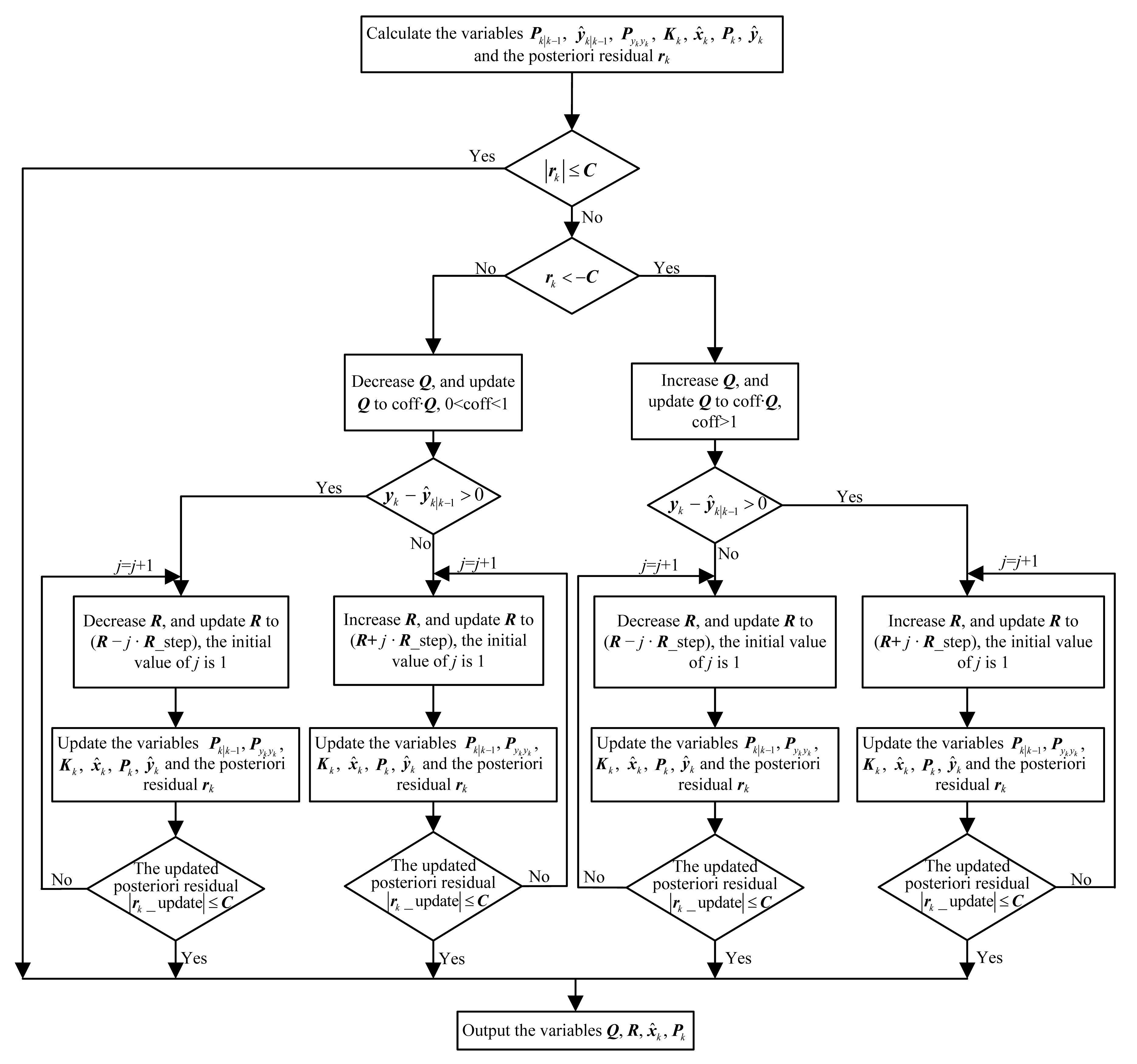
Therefore, we propose a novel adaptive UKF algorithm, in which the process noise covariance matrix Q and the measurement noise covariance matrix R can be tuned dynamically to obtain better performance of the filter. A flow chart of the adaptive law is shown in Fig. 1, and a description is presented below.

Fig.1
A flow chart of the adaptive law

The a posteriori mean ${{\mathbf{\hat x}}_k}$ can be acquired after measurement updating, and then the a posteriori estimate ${{\mathbf{\hat y}}_k}$ of the measurement vector is obtained as (23) ${{\mathbf{\hat y}}_k} = h({{\mathbf{\hat x}}_k})$ .

Here, we define a variable r _k which is the a posteriori residual between the actual measurement value and the a posteriori estimate: (24) ${{\mathbf{r}}_k} = {{\mathbf{y}}_k} - {{\mathbf{\hat y}}_k}$ .

A positive threshold value ( C ) is preset. If the absolute value of the a posteriori residual r _k is less than the preset threshold value C , it means the residual is within an acceptable range and the a posterior estimate ${{\mathbf{\hat y}}_k}$ is approximately equal to the actual measurement value y _k . That is to say, the two parameters Q and R are satisfactory and do not need adjustment. If the a posteriori residual r _k is less than − C , it means the a posteriori estimate ${{\mathbf{\hat y}}_k}$ is more than the actual measurement value y _k , and the deviation exceeds the preset threshold C . The a posteriori estimate ${{\mathbf{\hat y}}_k}$ can be reduced to a value close to the actual measurement value y _k by the following method. The method is to increase Q and R when the a priori residual $({{\mathbf{y}}_k} - {{\mathbf{\hat y}}_{\left. k \right|k - 1}})$ is larger than zero and decrease R when the a priori residual $({{\mathbf{y}}_k} - {{\mathbf{\hat y}}_{\left. k \right|k - 1}})$ is less than zero. If the a posteriori residual r _k is greater than C , it means the actual measurement value y _k is more than the a posteriori estimate ${{\mathbf{\hat y}}_k}$ and the deviation exceeds the preset threshold C . Therefore, the a posteriori estimate ${{\mathbf{\hat y}}_k}$ is needed to increase to a value approximately equal to the actual measurement value y _k . The approach to increase ${{\mathbf{\hat y}}_k}$ is to decrease Q and R when the a priori residual $({{\mathbf{y}}_k} - {{\mathbf{\hat y}}_{\left. k \right|k - 1}})$ is larger than zero and increase R when the a priori residual $({{\mathbf{y}}_k} - {{\mathbf{\hat y}}_{\left. k \right|k - 1}})$ is less than zero. After this adjustment, the absolute value of the updated a posteriori residual goes back to a value that is less than or equal to the preset threshold value C .

As mentioned above, if r _k <−C, Q is increased by multiplying a fix rate (coff) greater than 1. For R adjustment, if the a priori residual $({{\mathbf{y}}_k} - {{\mathbf{\hat y}}_{\left. k \right|k - 1}})$ is larger than zero, R is increased; and if the a priori residual $({{\mathbf{y}}_k} - {{\mathbf{\hat y}}_{\left. k \right|k - 1}})$ is less than zero, R is decreased. Whether increasing or decreasing R , a step R _step is set first, and then we can search with the step size to find an appropriate R so that the absolute value of the a posteriori residual is less than or equal to the preset threshold value C . If r _k >C, the adjustment method is similar to the above. For Q adjustment, Q is decreased by multiplying a fix rate (coff) which is chosen to be between 0 and 1. For R adjustment, if the a priori residual $({{\mathbf{y}}_k} - {{\mathbf{\hat y}}_{\left. k \right|k - 1}})$ is larger than zero, R is decreased; and if the a priori residual $({{\mathbf{y}}_k} - {{\mathbf{\hat y}}_{\left. k \right|k - 1}})$ is less than zero, R is increased. The adjustment method of R is the same as the above and a step R _step is also set first. By adjustment of Q and R , the absolute value of the updated a posteriori residual goes back to a value that is less than or equal to the preset threshold value C .

The variables ${{\mathbf{\hat x}}_k}$ , P _k , Q , and R are updated dynamically according to the adaptive UKF algorithm within the identifying time LΔt, to give values which are closer to the practical values. However, there are no actual measurement values after the identifying time, thus we cannot adjust Q and R because the adaptive law relies on real measurement values. After the identifying time, the normal UKF algorithm is used to predict the variables ${{\mathbf{\hat x}}_k}$ , ${{\mathbf{P}}_k}$ , and ${{\mathbf{\hat y}}_k}$ , and Q and R are maintained as the last values modified in the identifying time.

2.3. Temperature rise model

According to thermal modal theory (Matsuo et al., ; Xia et al., ), for a thermal system, we can indicate its transient conduction problem using the following equation: (25) $[{\mathbf{C}}]\left\{ {\frac{{{\text{d}}{\mathbf{\theta }}}}{{{\text{d}}t}}} \right\} + [{\mathbf{H}}]\{ {\mathbf{\theta }}\} = \{ {\mathbf{P}}\}$ , where [ C ], [ H ], and { P } are the heat capacity matrix, the heat conductive matrix, and the heat source strength vector, respectively; and { θ } is the temperature vector.

The solution of Eq. (25) can be calculated by solving the equation as follows: (26) $[{\mathbf{H}}]{\{ {\mathbf{M}}\} _j} = {\lambda _j}[{\mathbf{C}}]{\{ {\mathbf{M}}\} _j},\;\;\;\;{\text{ }}j = 1,\;2,\; \cdots ,p$ , where { M } _j is the characteristic mode vector, and λ_j is the thermal eigenvalue.

Then, the expression of the solution of Eq. (25) is (27) $\{ {\mathbf{T}}\} = \sum\limits_{j = 1}^p {{{\{ {\mathbf{M}}\} }_j}\{ {\mathbf{M}}\} _j^{\text{T}}} \int_0^t {\{ {\mathbf{P}}(\tau )\} } {{\text{e}}^{ - {\lambda _j}(t - \tau )}}{\text{d}}\tau + \sum\limits_{j = 1}^p {{{\{ {\mathbf{M}}\} }_j}\{ {\mathbf{M}}\} _j^{\text{T}}[{\mathbf{C}}]\{ {{\mathbf{T}}_0}\} } {{\text{e}}^{ - {\lambda _j}t}}$ , where { T ₀} is the initial temperature. When { T ₀}={0} and { P (τ)} is a step loading, Eq. (27) can be simplified as (28) $\{ {\mathbf{T}}\} = \sum\limits_{j = 1}^p {\frac{1}{{{\lambda _j}}}{{\{ {\mathbf{M}}\} }_j}\{ {\mathbf{M}}\} _j^{\text{T}}} \{ {{\mathbf{P}}_0}\} - \sum\limits_{j = 1}^p {\frac{1}{{{\lambda _j}}}{{\{ {\mathbf{M}}\} }_j}\{ {\mathbf{M}}\} _j^{\text{T}}} \{ {{\mathbf{P}}_0}\} {{\text{e}}^{ - {\lambda _j}t}}$ .

Therefore, Eq. (28) can be turned into a more compact form (29) ${\mathbf{T}}(r,\;t) = {{\mathbf{T}}_\infty }(r) + \sum\limits_{j = 1}^p {{{\mathbf{D}}_j}(r){{\text{e}}^{ - {\lambda _j}(r)t}}}$ , where r is the position coordinates of a measuring point, T (r, t) is the transient temperature of the measuring point in location r at time t, T _∞ (r) is the steady state temperature of the measuring point in location r, D _j (r) is a constant which is related to the thermophysical properties of the material and initial temperature, λ_j (r) is also a constant which is related to comprehensive physical properties of the thermal system, t is a time variable, and j=1, 2, …, p denotes there are p terms. We can use Eq. (29) to indicate the transient temperature distribution of the thermal system. When temperature is measured without external disturbance, the high order terms from 2 to p decay rapidly. So we retain the first term to approximately represent the transient temperature distribution: (30) ${\mathbf{T}}(r,t) = {{\mathbf{T}}_\infty }(r) + {\mathbf{D}}(r){{\text{e}}^{ - \lambda (r)t}}$ .

The temperature rise model is transformed into a discrete state-space model form. Assume state vector x =[T λ T _∞]^T, and the discrete temperature rise model is expressed in the following form: (31) ${{\mathbf{x}}_k} = f({{\mathbf{x}}_{k - 1}}) + {{\mathbf{w}}_{k - 1}} = \left[ {\begin{array}{*{20}{c}} {{T_{\infty ,k - 1}} + ({T_{k - 1}} - {T_{\infty ,k - 1}}){{\text{e}}^{ - {\lambda _{k - 1}} \cdot \Delta t}}} \\ {{\lambda _{k - 1}}} \\ {{T_{\infty ,k - 1}}} \end{array}} \right] + {{\mathbf{w}}_{k - 1}}$ , (32) ${{\mathbf{y}}_k} = h({{\mathbf{x}}_k}) + {{\mathbf{v}}_k} = {{\mathbf{T}}_k} + {{\mathbf{v}}_k}$ , where Δt is the sampling interval, and k denotes the moment at time kΔt.

2.4. Fast identification of a machine tool selected point temperature rise

The machine tool selected point temperature rise curve can be obtained through the adaptive UKF algorithm within the identifying time, and through the normal UKF algorithm after the identifying time. To characterize the accuracy of the prediction, we use a new variable root mean square error (RMSE) between the estimated temperature and the measured temperature in a given period of time: (33) $\sigma = \sqrt {\sum\limits_{k = 1}^M {{{[{T_{\text{e}}}(k) - {T_{\text{o}}}(k)]}^2}/(M - 1)} }$ , where σ is the RMSE; M is the total number of measuring times, MΔt represents the measuring time; T _e(k) is the estimated temperature at time kΔt; and T _o(k) is the measured temperature at time kΔt.

Here, the measuring time MΔt is defined as the sampling time, and the identifying time must be less than the sampling time.

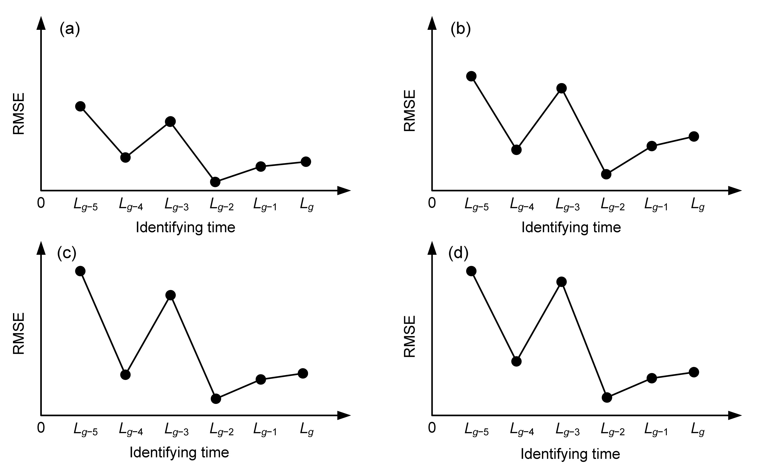
Assume first that temperature is measured during a sampling time M ₁Δt, and an identifying time L ₁Δt is chosen. The temperature of a selected point is estimated and the variables ${{\mathbf{\hat x}}_k}$ , P _k , Q , and R are updated dynamically by use of the actual measured temperature, according to the adaptive UKF algorithm within the identifying time L ₁Δt. After the identifying time L ₁Δt, the selected point temperature is predicted according to the normal UKF algorithm. The machine tool selected point temperature rise curve can be obtained through the above process. To evaluate the accuracy of prediction, the RMSE between the predicted temperature and the measured temperature in a sampling time M ₁Δt is chosen. The RMSE is denoted by σ ₁. Draw a figure with the identifying time as the horizontal coordinate and the RMSE in a period of sampling as the vertical coordinate. The symbol (L ₁, σ ₁) denotes the point with the identifying time L ₁Δt as the abscissa and the RMSE σ ₁ as the ordinate. Then the point (L ₁, σ ₁) is drawn in the figure. When the identifying times L ₂Δt, …, L_g Δt are chosen and L ₁<L ₂<…<L_g <M, the corresponding curves of temperature rise at each selected point are obtained. Different RMSEs σ ₂, …, σ_g between the estimated temperature and the measured temperature in the same sampling period M ₁Δt can be obtained in the same way. The points (L ₂, σ ₂), …, (L_g , σ_g ) are shown in Fig. 2a, which shows the change in RMSE with different identifying times in sampling period M ₁Δt.

Fig.2
Changes in RMSE with different identifying times in different sampling periods: (a) M ₁Δt; (b) M ₂Δt; (c) M ₃Δt; (d) M ₄Δt

When the sampling period is increased to M ₂Δt, different RMSEs σ ₁′, σ ₂′, …, σ_g ′ with different identifying times L ₁Δt, L ₂Δt, …, L_g Δt can be calculated. These points (L ₁, σ ₁′), (L ₂, σ ₂′), …, (L_g , σ_g ′) are drawn in Fig. 2b, which shows the change in RMSE with different identifying times in sampling period M ₂Δt. Similarly, Fig. 2c represents the change in RMSE with different identifying times in sampling period M ₃Δt, and Fig. 2d the RMSE change with different identifying times in sampling period M ₄Δt.

For each of the four sampling times, the RMSE is minimal with the same identifying time, L_g ₋₂Δt. If this identifying time is found, the measurement test can be stopped and the identifying time is called the minimal time for identification. From this we can predict the selected point temperature rise accurately. In this way, the time of temperature rise test can be greatly reduced.

For a certain identifying time with a certain sampling period, the temperature rise of the selected point can be predicted according to the novel adaptive UKF algorithm within the identifying time, and according to the normal UKF algorithm after the identifying time. Furthermore, the RMSE between the estimated temperature and the measured temperature in the sampling period can be calculated. Then, RMSEs for different identifying times and sampling periods can also be obtained and the minimal time for identification can be searched according to the above process. When the minimal time for identification is found, the measurement test can be stopped and the selected point temperature rise can be predicted accurately. The minimal time for identification is always short, around 30 min. In practice, it takes 3–6 h or even longer to obtain a selected point temperature rise from the start-up of a machine tool until a steady-state temperature is reached. Therefore, the presented method for selected point temperature rise identification based on a novel adaptive UKF can be applied to greatly decrease the time taken to obtain the temperature rise curve. The method has good prospects for industrial application.

3. Tests on a vertical machining center

3.1. Application of the fast identification method based on the adaptive UKF

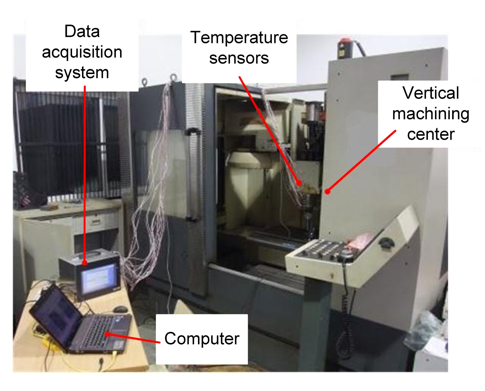
A vertical machining center was used to validate the effectiveness of the fast identification of machine tool selected point temperature rise based on the novel adaptive UKF algorithm. Fig. 3 shows the equipment of the temperature rise test system, which included four parts: a vertical machining center, several temperature sensors, a data acquisition system, and a computer. Several temperature sensors were arranged at different positions in the vertical machining center to measure temperature. The measured temperature data were recorded by the data acquisition system and then processed and analyzed in the computer. The process of fast selected point temperature rise identification based on the adaptive UKF was performed on the computer. All temperature sensors were of the PT100 type.

Fig.3
Temperature rise test system

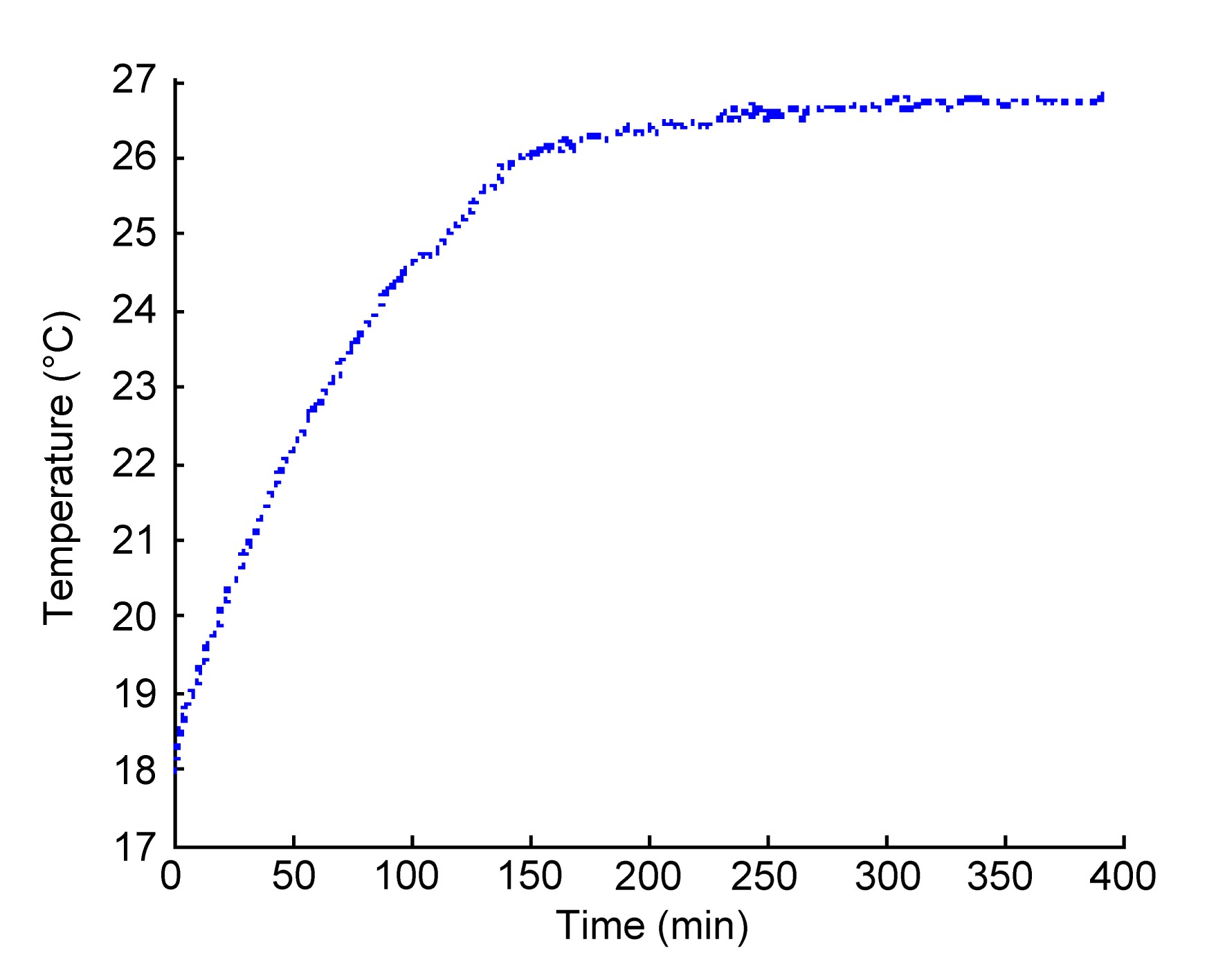
The room temperature was about 17.9 °C. When the vertical machining center started and the spindle was running at a speed of 5000 r/min, the temperature rise test began. The sampling interval Δt was set to 1 min. Thus, temperature measuring data were recorded every minute until the machine tool reached a steady-state temperature. The process for rapidly identifying a selected point temperature rise can be illustrated by taking one point as an example. Temperature rise curves of other points can be predicted in the same way. Fig. 4 shows the measured temperature of the selected point. The total measuring time was 394 min.

Fig.4
Measured temperature of a selected point

First, some parameters needed to be initialized. The initial state vector of the temperature rise model was chosen as x ₀=[T ₀ λ ₀ T _∞,0]^T=[10 0.01 30]^T, the mean value of the initial state vector as ${{\mathbf{\hat x}}_0} = {{\mathbf{x}}_0}$ , the covariance of the initial state vector as P ₀=diag(0.5², 0.1², 0.1²), the initial covariance matrix Q of the process noise as Q ₀=diag(0.001², 0.001², 0.001²), the initial covariance matrix R of the measurement noise as R ₀=0.001², the initial standard deviation q of the process noise as q ₀=diag(0.001, 0.001, 0.001), and the initial standard deviation r of the measurement noise as r ₀=0.001. In the adaptive law, when the covariance matrix Q of the process noise needs to be increased, the fix rate coff is set to 10, that is to say, Q _update = 10 Q ; when Q needs to be decreased, the fix rate coff is set to 0.1, in other words, Q _update=0.1 Q . The parameter R _step was set to R /100. The preset threshold C was chosen as 0.0001.

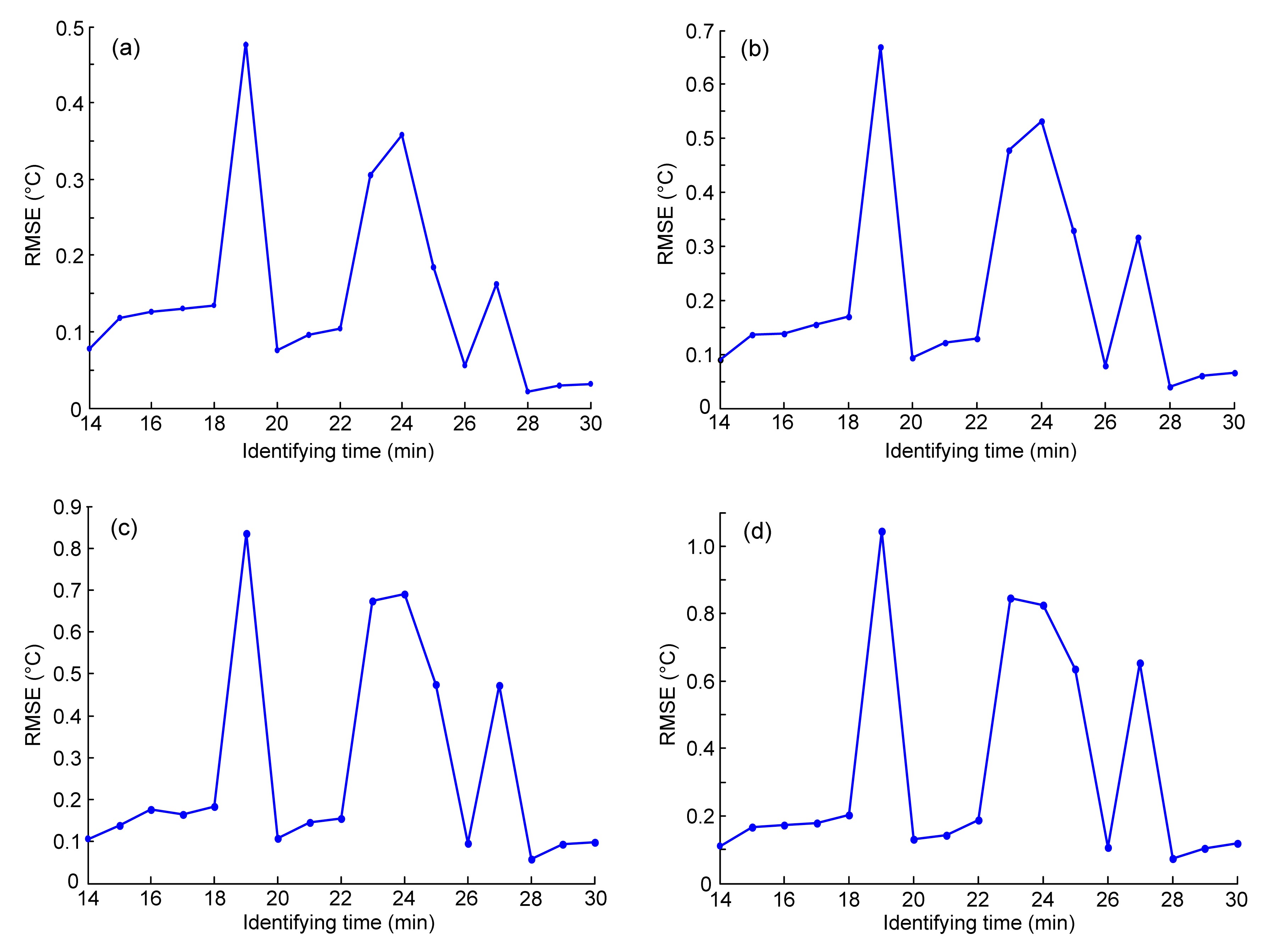
According to the above method, Figs. 5a–5d show the change in the RMSE curve corresponding to different sampling times of 35, 40, 45, and 50 min, respectively. From these four figures, we can easily see that the RMSE is minimal at the same identifying time of 28 min. Therefore, the selected point temperature rise can be predicted accurately within 28 min. If the present method is not applied, it takes 394 min of measuring time to obtain the selected point temperature rise from the start-up of the machine tool to the time it reaches a steady-state temperature.

Fig.5
Changes in RMSE with identifying times for different sampling periods of the selected point: (a) 35 min; (b) 40 min; (c) 45 min; (d) 50 min

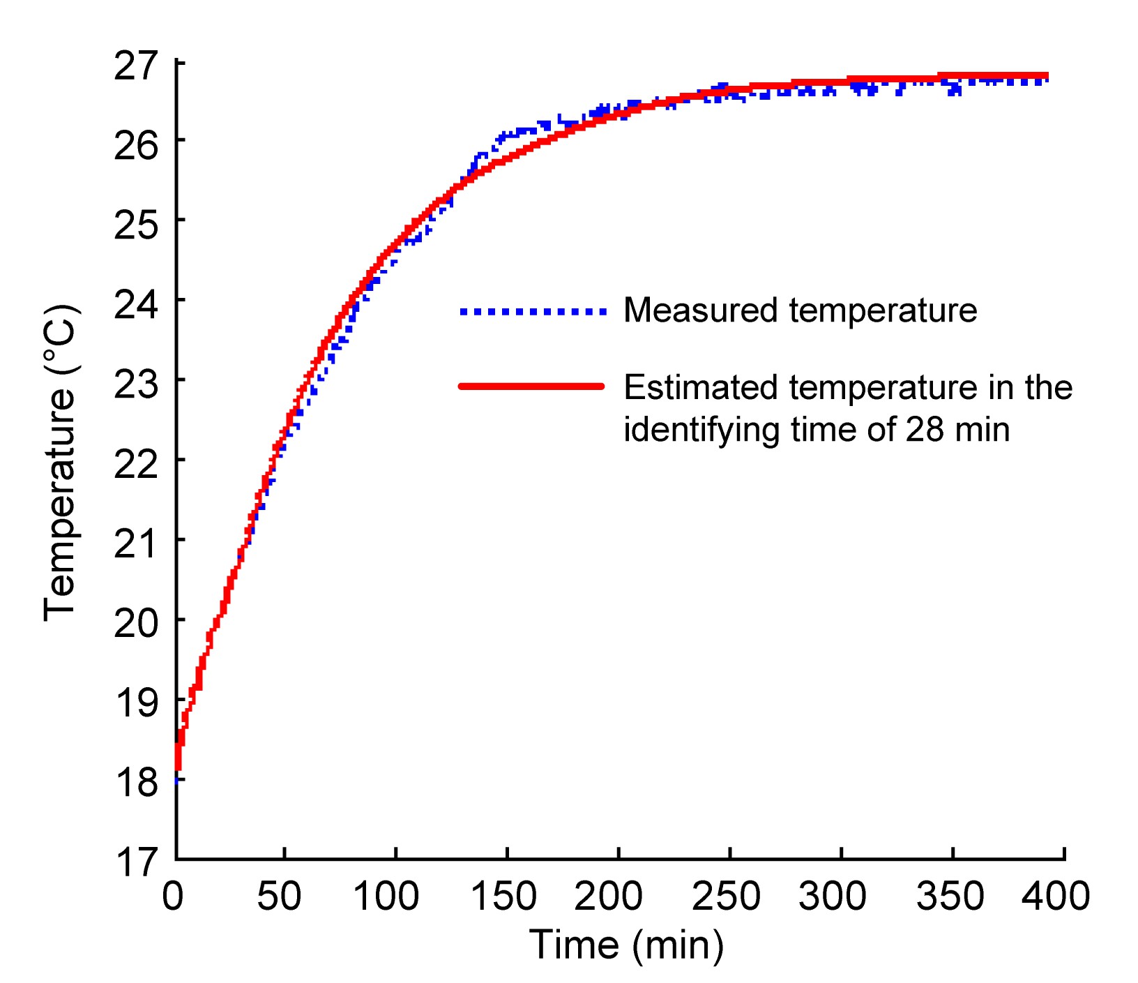
In the identifying time of 28 min, the adaptive UKF algorithm was adopted to identify the selected point temperature rise. The parameters Q and R were adjusted to diag(10⁻⁷, 10⁻⁷, 10⁻⁷) and 1.932×10⁻⁹, respectively. Fig. 6 shows the predicted temperature rise curve in the identifying time of 28 min and the measured temperature rise curve. We used the steady-state temperature and thermal equilibrium time to compare the estimated and measured temperature rises of the selected point. When the temperature reaches 95% of the maximum temperature rise, this state is called the thermal equilibrium state, and that moment the thermal equilibrium time. The estimated steady-state temperature was 26.797 °C, and the thermal equilibrium time was 197 min. The measured steady-state temperature was 26.7 °C, and the thermal equilibrium time 195 min. So the selected point temperature rise identified by the proposed method was satisfactory.

Fig.6
Measured and estimated temperature rises of the selected point based on UKF with model adaptation

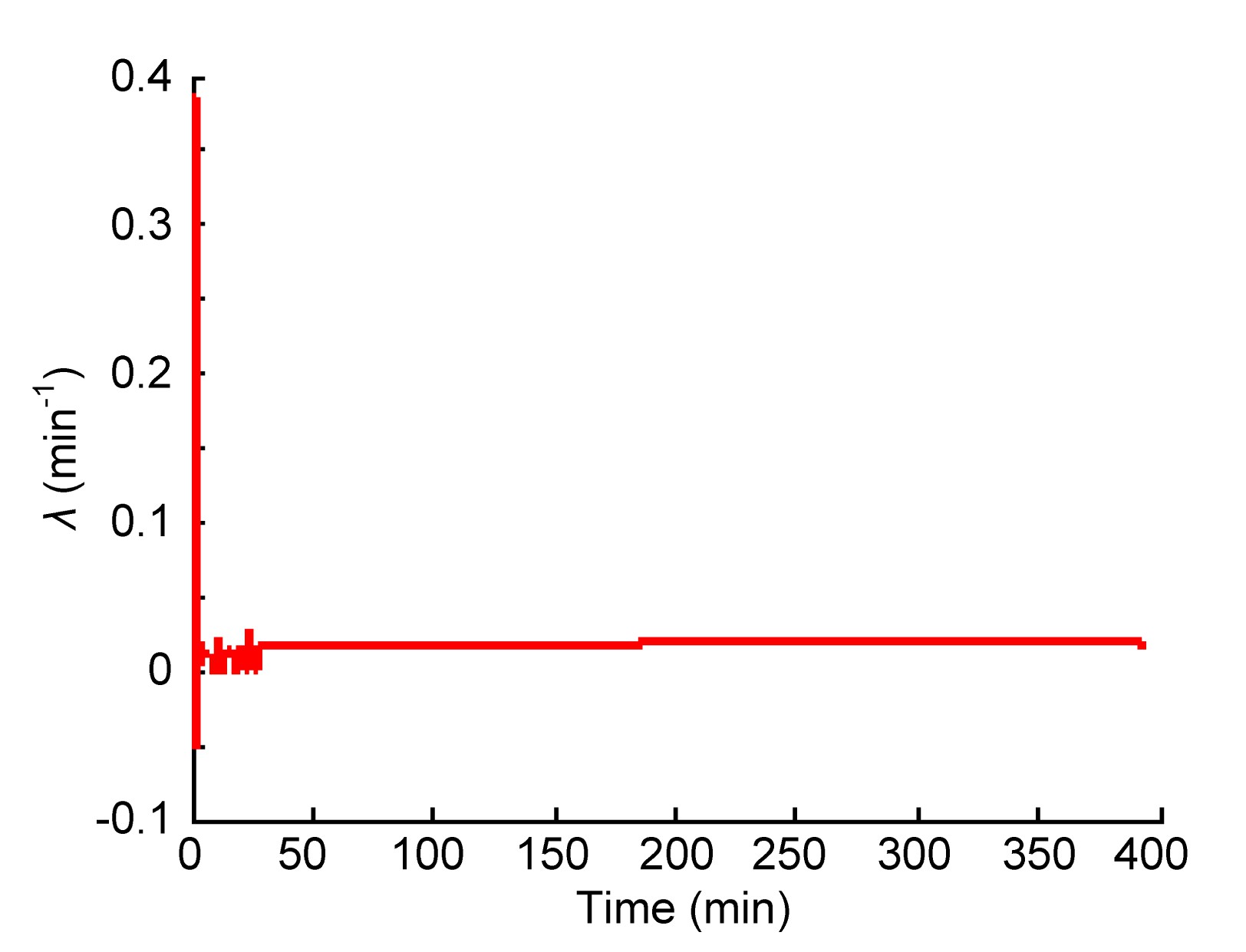
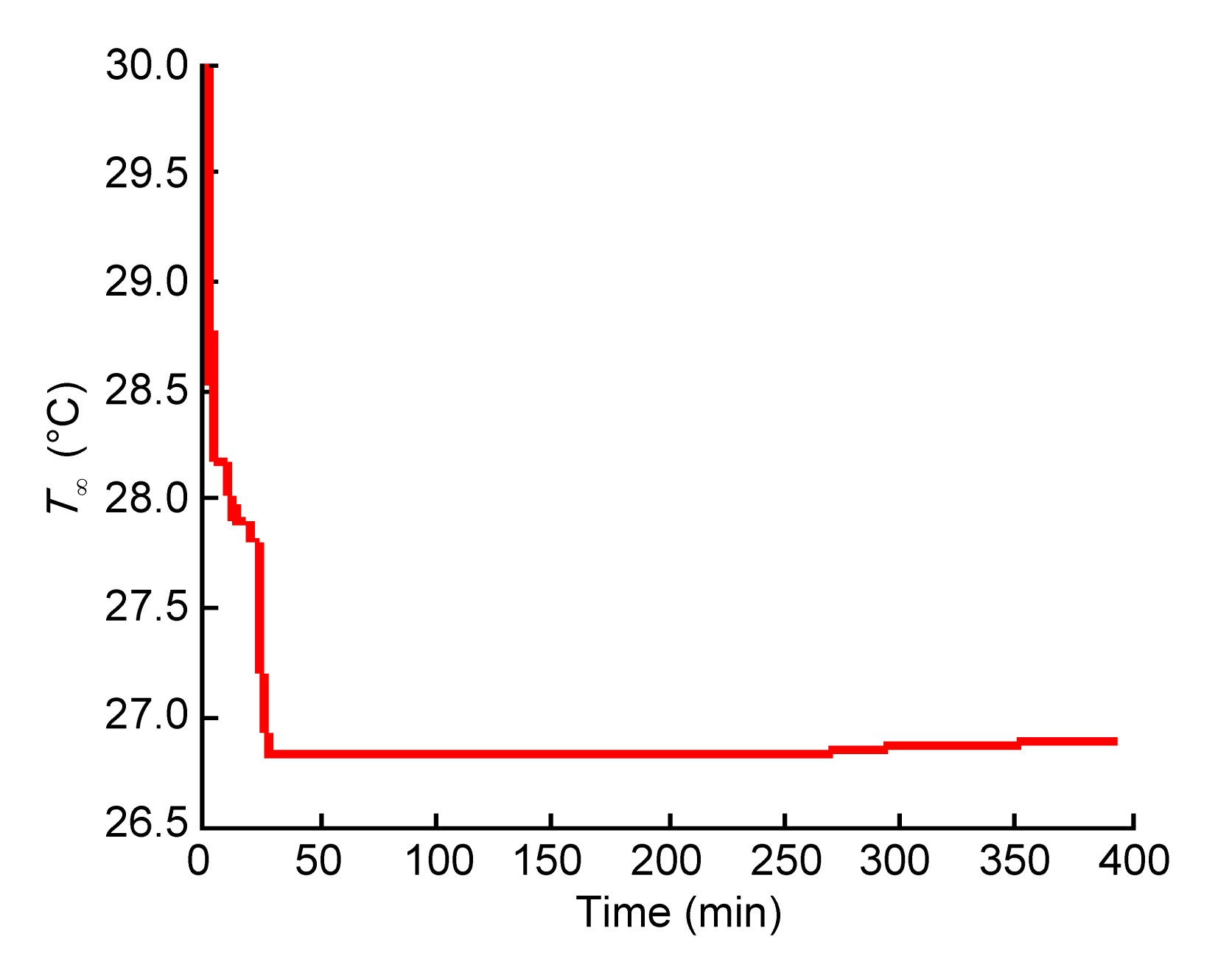
For the state vector x =[T λ T_∞ ]^T, the parameters λ and T_∞ are also obtained in the process of identifying the temperature rise. Figs. 7 and 8 show the estimated λ and T_∞ , respectively. The estimated variable λ converges to 0.016 min⁻¹ in Fig. 7, and the estimated variable T_∞ converges to 26.797 °C in Fig. 8.

Fig.7
Estimated variable λ

Fig.8
Estimated variable T_∞

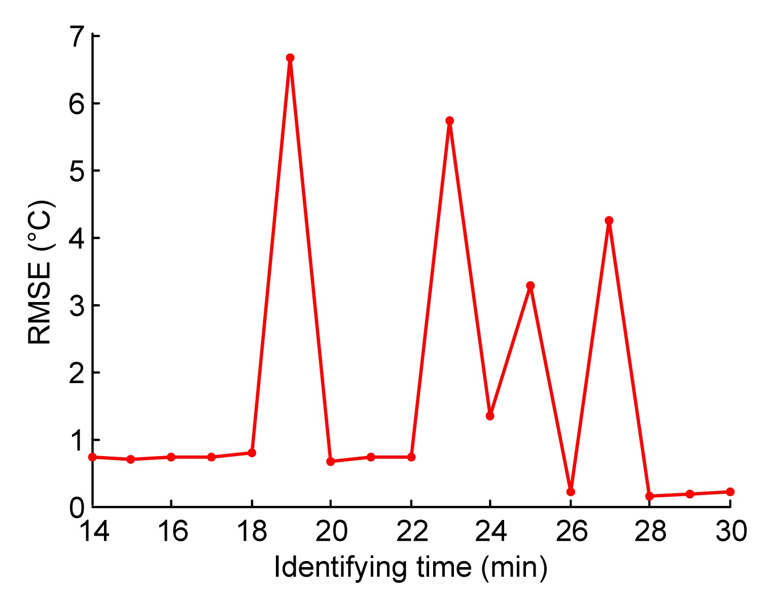
Then, we can calculate the RMSEs between the predicted and measured temperatures with different identifying times in the period of time from the start-up of the machine tool to the time a steady-state temperature is reached (394 min). Fig. 9 shows the change in RMSE with different identifying times with a sampling period of 394 min. The minimal RMSE (0.1291 °C) was found in the identifying time of 28 min. This time was the same as that based on the fast identification of the selected point temperature rise. Therefore, the proposed method for fast identification of the selected point temperature rise is effective.

Fig.9
Changes in RMSE with different identifying times in a sampling period of 394 min

3.2. A comparison of results from the unscented Kalman filter with and without model adaptation

Next, a comparison of the selected point temperature rise identification based on adaptive UKF and UKF without the adaptive algorithm is presented. In the process of identifying the selected point temperature rise based on UKF without the adaptive algorithm, the same initial parameters were used:

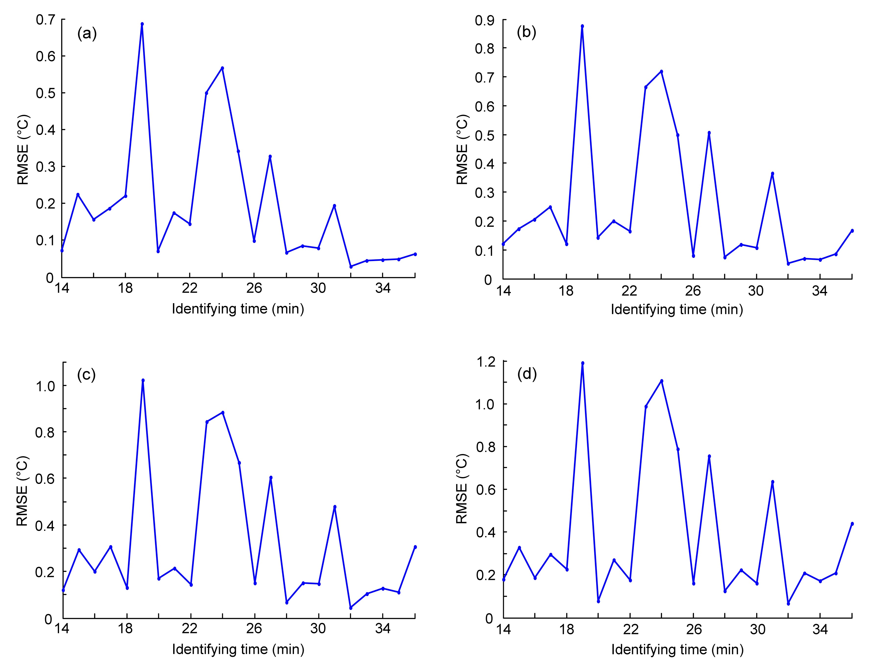
${\kern 0pt} \begin{matrix} {{{\mathbf{\hat x}}}_0} = {{\mathbf{x}}_0} = \begin{array}{*{20}{c}} {[{T_0}}\quad {{\lambda _0}}\quad {{T_{\infty ,0}}} \end{array}{]^{\text{T}}} = {[\begin{array}{*{20}{c}} {10}\quad {0.01}\quad {30} \end{array}]^T}, \hfill \\ {{\mathbf{P}}_0} = {\text{diag(}}{0.5^2},\;{0.1^2},\;{0.1^2}), \hfill \\ {{\mathbf{Q}}_0} = {\text{diag}}({0.001^2},\;{0.001^2},\;{0.001^2}), \hfill \\ {{\mathbf{R}}_0} = {0.001^2}, \hfill \\ {{\mathbf{q}}_0} = {\text{diag(}}0.001,\;0.001,\;0.001), \hfill \\ {{\mathbf{r}}_0} = 0.001. \hfill \\ \end{matrix}$

Using the fast identification method based on UKF without the adaptive algorithm, the changes in RMSE with different identifying times in different sampling periods can be calculated. Figs. 10a–10d represent the change in the RMSE curves corresponding to sampling periods of 40, 45, 50, and 55 min, respectively. These four figures show that the RMSE is minimal in the same identifying time of 32 min.

Fig.10
Changes in RMSE with identifying times for the selected point based on the UKF without model adaptation in different sampling times: (a) 40 min; (b) 45 min; (c) 50 min; (d) 55 min

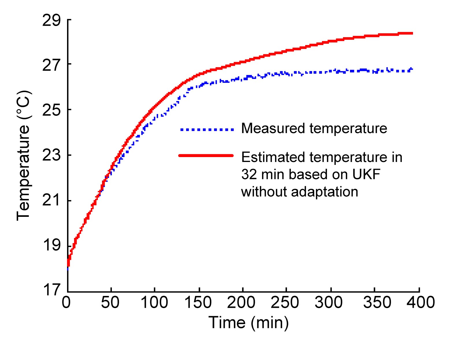
Fig. 11 shows the predicted temperature rise curve in the identifying time of 32 min based on UKF without adaptation and the measured temperature rise curve. Although there was a minimal identifying time of 32 min for the selected point using this method, the predicted temperature rise curve at 32 min deviated greatly from the measured temperature curve. However, the predicted temperature rise curve at 28 min based on the UKF with model adaptation was closer to the measured temperature (Fig. 6). For the unscented Kalman filter without adaptation, the covariance matrix Q of the process noise and covariance matrix R of the measurement noise remained unchanged so the covariances Q and R did not match the true covariances in the real system. This shows that the UKF without model adaptation suffers from performance degradation and even divergence. This is the reason why the estimated temperature curve in 32 min based on the UKF without adaptation deviated greatly from the measured temperature curve. When the UKF with model adaptation was used, the estimated temperature rise curve more closely matched the actual measurement temperature curve (Fig. 6). Therefore, the result of the selected point temperature rise identified by the UKF with model adaptation was satisfactory. The fast identification method based on the adaptive UKF has obvious advantages over the method without model adaptation.

Fig.11
Measured and estimated temperature rises of the selected point based on UKF without adaptation

4. Conclusions

In this paper, a novel method is presented for fast identification of a machine tool selected point temperature rise based on an adaptive UKF. The major advantage of the method is that it can predict the temperature rise in a short measuring time, like 30 min, instead of 3 to 6 h in conventional temperature rise tests. Moreover, the UKF algorithm can be successfully applied to temperature rise prediction for any measuring point, and modified to the adaptive UKF by adding the adaptive law. The adaptive UKF is used to decrease the influence of external perturbations on temperature rise prediction. A vertical machining center was used to validate the effectiveness of the presented method. In the experiment, taking one point as the selected point, the temperature rise of the selected point was identified in 28 min. The RMSE between the estimated and measured temperatures in the time period of 394 min was 0.1291 °C, and the error between the estimated and measured steady-state temperatures was 0.097 °C. So this method can effectively and quickly identify a machine tool selected point temperature rise.

* Project supported by the National Nature Science Foundation of China (No. 51175461), the Science Fund for Creative Research Groups of National Natural Science Foundation of China (No. 51221004), and the Specialized Research Fund for the Doctoral Program of Higher Education (No. 20120101110055), China

References

[1] Han, J., Wang, L.P., Wang, H.T., 2012. A new thermal error modeling method for CNC machine tools. International Journal of Advanced Manufacturing Technology, 62(1-4):205-212.

[2] He, W., Williard, N., Chen, C.C., 2013. State of charge estimation for electric vehicle batteries using unscented Kalman filtering. Microelectronics Reliability, 53(6):840-847.

[3] Hu, C., Chen, W., Chen, Y., 2003. Adaptive Kalman filtering for vehicle navigation. Journal of Global Positioning Systems, 2(1):42-47.

[4] Jiang, Z., Song, Q., He, Y.Q., 2007. A novel adaptive unscented Kalman filter for nonlinear estimation. . The 46th IEEE Conference on Decision and Control, New Orleans, USA, 5805-5810. :5805-5810.

[5] Julier, S.J., Uhlmann, J.K., 2004. Unscented filtering and nonlinear estimation. Proceedings of the IEEE, 92(3):401-422.

[6] Li, M.H., Hong, B.R., Luo, R.H., 2006. A novel method for mobile robot simultaneous localization and mapping. Journal of Zhejiang University-SCIENCE A, 7(6):937-944.

[7] Loebis, D., Sutton, R., Chudley, J., 2004. Adaptive tuning of a Kalman filter via fuzzy logic for an intelligent AUV navigation system. Control Engineering Practice, 12(12):1531-1539.

[8] Matsuo, M., Yasui, T., Inamura, T., 1986. High-speed test of thermal effects for a machine-tool structure based on modal-analysis. Precision Engineering, 8(2):72-78.

[9] Mayr, J., Jedrzejewski, J., Uhlmann, E., 2012. Thermal issues in machine tools. CIRP Annals-Manufacturing Technology, 61(2):771-791.

[10] Minase, J., Lu, T.F., Cazzolato, B., 2010. Adaptive identification of hysteresis and creep in piezoelectric stack actuators. International Journal of Advanced Manufacturing Technology, 46(9-12):913-921.

[11] Regulski, P., Terzija, V., 2012. Estimation of frequency and fundamental power components using an unscented Kalman filter. IEEE Transactions on Instrumentation and Measurement, 61(4):952-962.

[12] Uhlmann, E., Hu, J., 2012. Thermal modelling of a high speed motor spindle. . Fifth CIRP International Conference on High Performance Cutting, Zurich, Switzerland, 313-318. :313-318.

[13] Wan, E.A., van der Merwe, R., 2000. The unscented Kalman filter for nonlinear estimation. . Symposium on Adaptive Systems for Signal Processing, Communications, and Control, Mcmaster University, Lake Louise, Canada, 153-158. :153-158.

[14] Wu, M.L., Smyth, A.W., 2007. Application of the unscented Kalman filter for real-time nonlinear structural system identification. Structural Control & Health Monitoring, 14(7):971-990.

[15] Xia, C.H., Fu, J.Z., Xu, Y.T., 2014. Machine tool selected point temperature rise identification based on operational thermal modal analysis. International Journal of Advanced Manufacturing Technology, 70(1-4):19-31.

[16] Xing, Y.J., He, W., Pecht, M., 2014. State of charge estimation of lithium-ion batteries using the open-circuit voltage at various ambient temperatures. Applied Energy, 113:106-115.

[17] Zhang, J.F., Feng, P.F., Chen, C., 2013. A method for thermal performance modeling and simulation of machine tools. International Journal of Advanced Manufacturing Technology, 68(5-8):1517-1527.

[18] Zhao, H.T., Yang, J.G., Shen, J.H., 2007. Simulation of thermal behavior of a CNC machine tool spindle. International Journal of Machine Tools & Manufacture, 47(6):1003-1010.

Open peer comments: Debate/Discuss/Question/Opinion

<1>

Similar articles

- Go to