Chao-bang Yao, Wen-cai Dong. A fast integration method for translating-pulsating source Green’s function in Bessho form[J]. Journal of Zhejiang University Science A, 2014, 15(2): 108-119.
@article{title="A fast integration method for translating-pulsating source Green’s function in Bessho form", author="Chao-bang Yao, Wen-cai Dong", journal="Journal of Zhejiang University Science A", volume="15", number="2", pages="108-119", year="2014", publisher="Zhejiang University Press & Springer", doi="10.1631/jzus.A1300209" }
%0 Journal Article %T A fast integration method for translating-pulsating source Green’s function in Bessho form %A Chao-bang Yao %A Wen-cai Dong %J Journal of Zhejiang University SCIENCE A %V 15 %N 2 %P 108-119 %@ 1673-565X %D 2014 %I Zhejiang University Press & Springer %DOI 10.1631/jzus.A1300209
TY - JOUR T1 - A fast integration method for translating-pulsating source Green’s function in Bessho form A1 - Chao-bang Yao A1 - Wen-cai Dong J0 - Journal of Zhejiang University Science A VL - 15 IS - 2 SP - 108 EP - 119 %@ 1673-565X Y1 - 2014 PB - Zhejiang University Press & Springer ER - DOI - 10.1631/jzus.A1300209
Abstract: The singularities and oscillatory performance of translating-pulsating source Green’s function in Bessho form were analyzed. Relative numerical integration methods such as Gaussian quadrature rule, variable substitution method (VSM), and steepest descent integration method (SDIM) were used to evaluate this type of Green’s function. For SDIM, the complex domain was restricted only on the θ-plane. Meanwhile, the integral along the real axis was computed by use of the VSM to avoid the complication of a numerical search of the steepest descent line. Furthermore, the steepest descent line was represented by the B-spline function. Based on this representation, a new self-compatible integration method corresponding to parametric t was established. The numerical method was validated through comparison with other existing results, and was shown to be efficient and reliable in the calculation of the velocity potentials for the 3D seakeeping and hydrodynamic performance of floating structures moving in waves.
Darkslateblue:Affiliate; Royal Blue:Author; Turquoise:Article
Article Content
1. Introduction
The frequency-domain Green’s function with forward speed in 3D deep water was derived by Haskind (1953), and its physical meaning is the velocity potential of the field point produced by the unit translating and pulsating source. It has been widely used in computing wave-induced ship motions and loads (Bailey et al., 2001; Chen and Wu, 2001; Fang and Chan, 2002; Du et al., 2005; 2012; Zakaria, 2006; 2009; Zong and Qian, 2012). The advantages of this Green’s function are an automatic fulfillment of the linearized free surface and radiation conditions, and the absence of mesh on the free surface avoiding reflection on the boundary. However, it is difficult to ensure calculation efficiency and accuracy. The numerical difficulties of the problem can essentially be traced to the complexity of the mathematical expression for the Green’s function, or more precisely of any of the three available alternative expressions for this fundamental function. Xu and Dong (2011) discussed three other forms of this function such as Bessho form (Bessho, 1977), Michell form (Miao et al., 1995) and Havelock form (Rahman, 1990), which were obtained by using elementary mathematics. The Havelock form is a single integral. There are some difficulties in calculation such as infinite discontinuity when the denominator of the integrand equals zero, a jump discontinuous node in the exponential integral function of the local disturbance part, and high-frequency oscillatory performance of the far-field wave-like part. The Michell form is not suitable for numerical analysis because part of the function is a double integral. The Bessho form is considered as the most suitable for calculations because it is expressed by a single integral of the elementary functions in the complex domain. This single integral expression has a definite advantage over the others, which are expressed by using the exponential integral functions E1 from the point of view of computational accuracy and speed (Iwashita and Ohkusu, 1989; 1992; Du and Wu, 1998; Du et al., 2005). On the other hand, the numerical integration must be performed in the complicated complex domain, and there are still some difficulties in calculation as follows: (1) an infinite discontinuity exists when the denominator of the integrand is zero; (2) high frequency oscillatory performance of the integrand is complicated.
Some numerical integration methods have been studied to dispose of such singularities and high frequency oscillatory performance. Iwashita and Ohkusu (1989; 1992) developed a special algorithm, named “numerical steepest descent method”, for evaluating Bessho form translating-pulsating source Green’s function. Originally this method was obtained by transforming the complex θ-plane to the complex M-plane, where the integration range was mapped to the half-infinite region. Following this transformation, Du (1996) and Du and Wu (1998) established a fast algorithm for calculating this form of Green’s function by employing the steepest descent path method together with a self-adaptive integration method. Brument and Delhommeau (1997), Maury (2001), and Maury et al. (2003) further studied the choice of step, start points, and common use of many descent lines for the steepest descent method. The steepest descent integration method (SDIM) on the M-plane makes the numerical search of the steepest descent line easy when θ approaches ±π/2. However, the presence of new branch cuts must be taken into consideration and this sometimes complicates the numerical search of the steepest descent line. To improve this computational method, Iwashita (1997) directly performed the integration on the θ-plane without any transformation to other complex planes. However, to do the calculation, the information about the saddle points and the cross points between the real axis and the steepest ascent line must be analyzed to avoid many wrong paths when the start point is located on the real axis. This may be sometimes a waste of time.
In this paper, the singularities, oscillatory performance and their contribution factors of the Bessho form Green’s function were analyzed systematically, aiming to propose a fast numerical integration method based on the SDIM. The efficiency and accuracy of these integration methods were validated by numerical results.
2. Single integral expression of translating-pulsating source Green’s function in Bessho form
Assuming the translating-pulsating source is traveling at a forward speed U and oscillating at a frequency ωe, (ξ, η, ζ) is the source point and (x, y, z) is the field point, then the 3D translating-pulsating source Green’s function can be expressed as
,
,
where
,
,
,
,
,
,
,
,
,
,
,
where r and r1 are distances to source point and its symmetry with respect to the free surface, respectively; k1 and k2 are non-dimensional wave numbers of the propagation waves; τ is Brard parameter; K0 is wave number; and g is the gravitational acceleration.
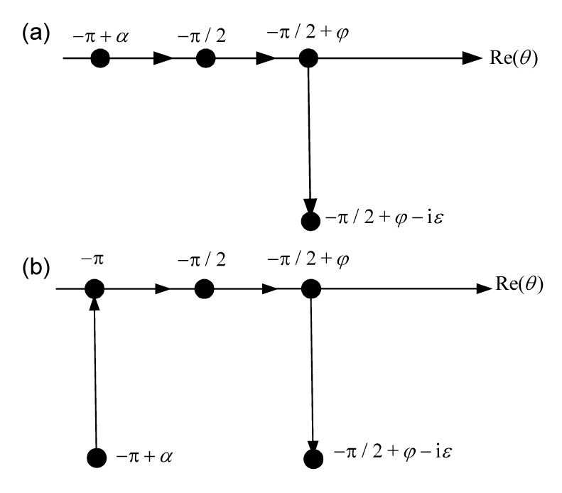
Integral paths of Bessho form Green’s function are shown in Fig. 1, where the symbols are defined as shown in Eq. (2).
Fig.1 Integral path: (a) corresponds to τ>0.25; (b) corresponds to τ<0.25
Despite the integral limits depending on the coordinates of the field points, differentiation of T with respect to x, y, and z is not as complicated as anticipated. The derivatives are listed as follows:
,
.
The integration methods for T presented in the following are also suitable for its three partial derivatives as given in Eq. (4), because no other calculation difficulties are added.
3. Characteristics of the integrand of T
3.1. Characteristics of ki
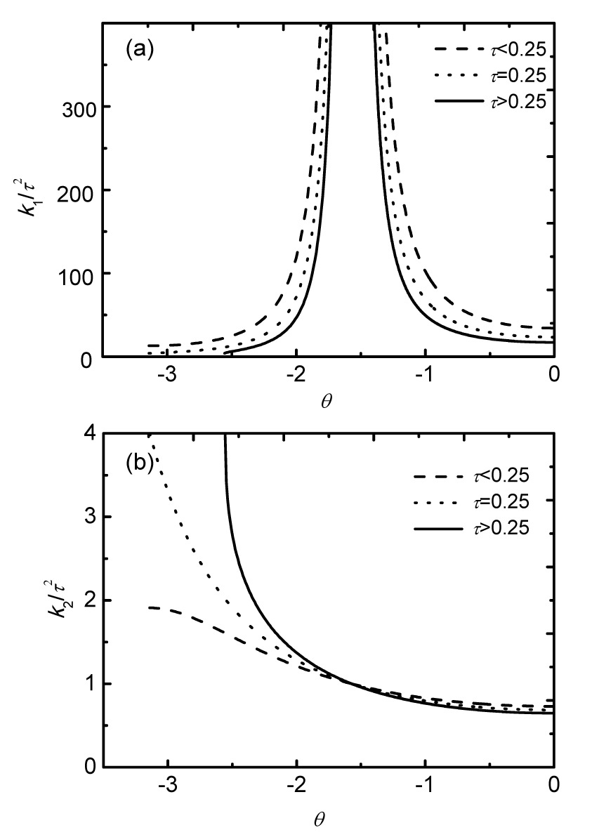
ki is the non-dimensional wave number of the propagation wave generated by the translating-pulsating source whose independent variables are τ and θ. ki is an important parameter of the integrands which influence performances of the propagation parts. Meanwhile, ki is also dependent on the definition domain of θ, which is defined by the relative position of field and source points. Typical function images of ki are presented in Fig. 2: if and if .
Fig.2 Typical images of k1/τ2 (a) and k2/τ2 (b)
Some findings for the characteristics of ki can be drawn as follows: (1) for , presents the tendency to infinity; as a result, the integrand oscillates with high frequency as θ approaches , which may be a big obstacle for numerical integration. (2) if , then , terms in k2 do not oscillate with high frequency, and numerical integration is straightforward. Due to their behavior, terms in k1 and k2 are computed differently.
From the point of numerical calculation, under conditions of , and k2 can be calculated according to Eq. (5), if (&kgr; is infinitely small),
3.2. Singularity and oscillatory behavior of the integrand
The integral limits of Eq. (2a) depend on τ and φ, the lower limit θ1 is complex or a real number corresponding to τ<0.25 or τ>0.25. When X≥0, φ∈[0, π/2]; when X<0, φ∈[π/2, π].
To investigate the behavior of the integrands, we separate the integral over θ into different parts according to the sign of terms sgnc.
where and
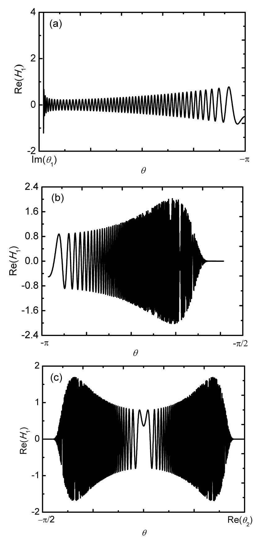
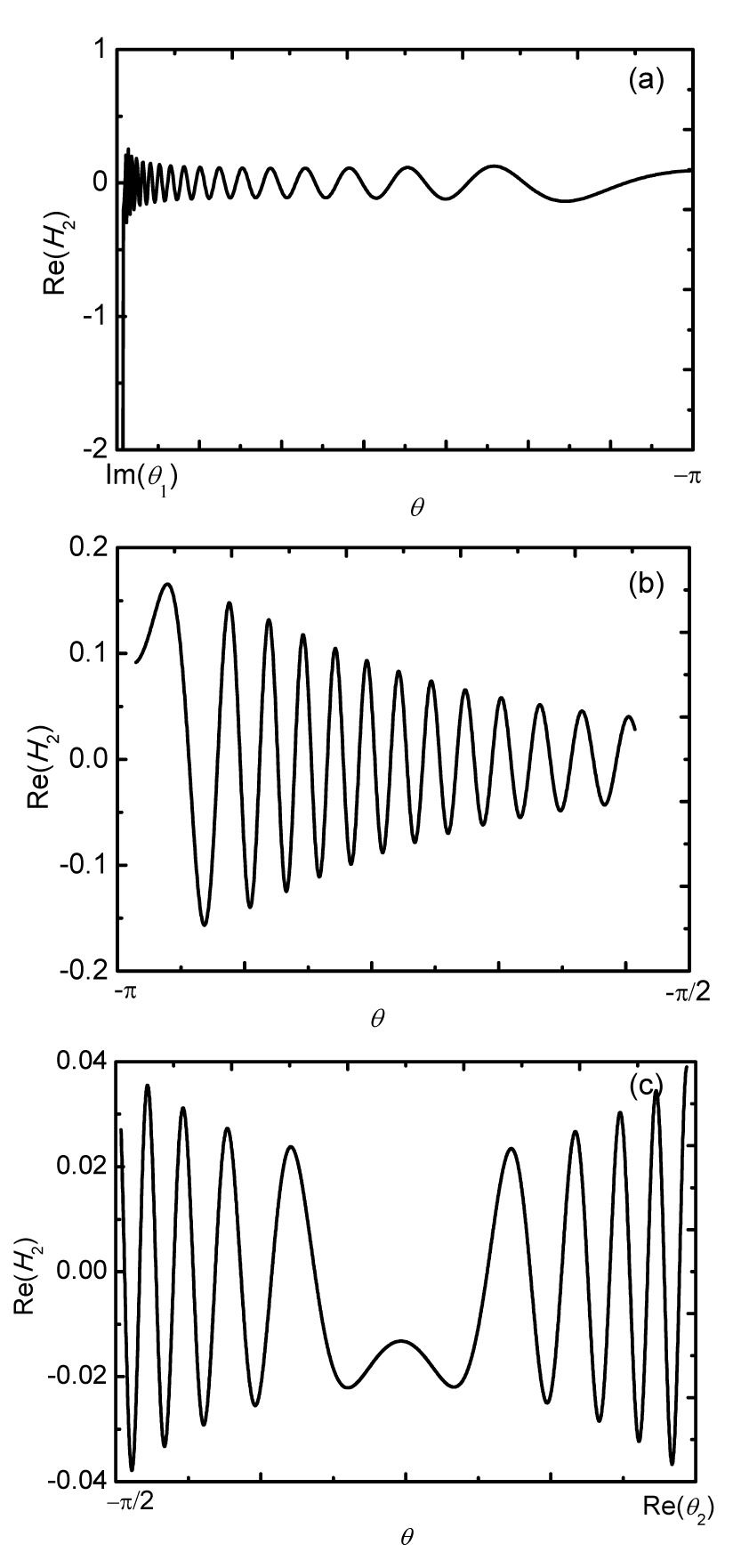
Fig. 3 and Fig. 4 show images of Hj(θ) when for τ=0.2, X=−500, Y=1, and Z=−0.2. The performance of the integrand in this case can be summarized as follows.
(1) It is certain that θ1 is an infinite discontinuity and values of terms in k1 and k2 change violently as θ approaches θ1.
(2) When , the performance of is oscillatory because of the complex exponential function (j=1, 2), which can be written as . The term determines the value of the oscillatory frequency and, the larger it is, the higher the frequency is. It can also be concluded that the value of determines whether is higher-frequency oscillatory with the condition of . The other part is an attenuation term (kjZ<0) and determines amplitudes of Hj. When is getting larger, the attenuation speed of Hj becomes higher. As for H2, the value of k2 is not as large as shown in Fig. 2, so only when the parameter ρ is very large can H2 act as high-frequency oscillatory. In addition, attenuation performance of H2 is not obvious because values of are not large either. As far as H1 is concerned, k1 is very large when , so H1 becomes high-frequency oscillatory not only when ρ is very large but also when . However, H1 attenuates very fast when θ approaches since is also very large and H1 becomes zero when .
Fig.3 Typical images of integrands corresponding to k1 (τ=0.2) (a) [Im(θ1), −π]; (b) [−π, −π/2]; (c) [−π/2, Re(θ2)]
Fig.4 Typical images of integrands corresponding to k2 (τ=0.2) (a) [Im(θ1), −π]; (b) [−π, −π/2]; (c) [−π/2, Re(θ2)]
4. Numerical integration methods
4.1. Integration methods for the singularities at terminals
From the analysis above, we can see that θ1 is an infinite jump discontinuous node of terms both in k1 and k2. Gaussian quadrature rule (Abramowitz and Stegun, 1964) is used in this study to eliminate such a node. However, this rule is not suitable to calculate the oscillatory function, so we apply it only within the domain [θ1, θd], where θd is defined by
.
In practice, is proved to be adequate.
By performing , and applying the Gaussian quadrature rule to Hj(θ) when its interval is [θ1, θd], the integral can be obtained approximately as follows:
,
where , , , , , , and m is the discrete step of the interval. μ(t) can be written as
The integral may be obtained by using the variable substitution method which will be discussed in detail as below, when the interval is (τ<0.25) or (τ>0.25).
4.2. Integration methods for θ within the domain of [θ1, −π/2]
It is inefficient and sometimes even impossible to calculate integrals in k1 and k2 by using usual integration methods because oscillation characteristics of these integrals are extremely complicated. The steepest descent method is often used to compute terms in k1; however, when the steepest descent line starts from the real axis, the search algorithm of these lines are often difficult and complicated. In this study, a method based on a variable substitution is introduced for the calculation.
4.2.1. Integration method for θ on the real axis
If the interval for Hj(θ) is the domain of [θe, θs], the integral of Hj(θ) can be written as Eq. (10) by performing .
,
where .
Performing , where l is a real part and d is an imaginary part. Substitute it into Eq. (10) and multiply it by l−id, then Eq. (10) can be converted into the following expression:
,
where
,
,
,
,
.
Integrands of Eq. (11) can be written as , where fj is a complex function and can be expressed as follows:
.
Assuming that the discrete sequences of [θe, θs] are , the relative sequences of Aj are Aj(θ1), Aj(θ2), …, Aj(θm).
If a linear function about Aj is used to approximate fj between Aj(θn) and Aj(θn+1) (), the integral In between the two points can be expressed as Eq. (14) through integration by parts
.
Thus, the sum of In approximates to the integral of Hj(θ) ([θe, θs]). The accuracy of this integration method is determined by the performance of fj and its relative interval discrete method. It is not difficult to prove that fj is continuous within the integration interval.
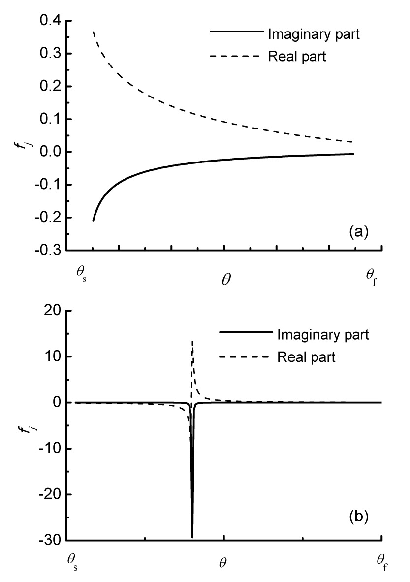
The completed variable substitution has transformed the oscillatory function into a formula easy for integration. It should be pointed out that values of fj vary violently in a narrow zone near relevant θf when d equals zero. θf is defined to be the root of equation d=0, which can be simplified as Eq. (15) by some mathematical derivations. It can be easily obtained that the root number of Eq. (15) is smaller than 2.
.
Fig. 5a gives typical curves of Re[fj] and Im[fj] when no root is existing in Eq. (15). The curves are smooth and easy to discrete. Typical curves of Re[fj] and Im[fj] with one root existing in Eq. (15) are given in Fig. 5b and the characteristics of these curves are:
(1) The curve shape of Im[fj] in the narrow zone near θf is leptokurtic;
(2) Values of Re[fj] change violently in the narrow zone around θf, and θf looks like a jump discontinuous node but it is a false appearance here because fj is continuous at the point of θf. This false appearance is defined as a false bizarre phenomenon and the respective θf is defined as a false singularity. The false bizarre phenomenon should be taken into account to improve the integration efficiency and accuracy during discrete treatment of the integral interval. At this point, the local refinement of the integral steps technique should be applied.
Fig.5 Typical characteristics of fj: (a) no root existing; (b) one root existing
4.2.2. Integration method for [θ1, −π] when τ<0.25
The Gaussian quadrature rule is applied to evaluate the integration within the domain [θ1, θd] (θd is defined as above), when τ<0.25. However, within the domain of [θd, −π] the integrands of Hj(θ) also have complicated oscillatory characteristics when ρ has a large value or the locations of source points and field points change. At this point, the method based on variable substitution is used again.
If the interval is [θe2, θs2], then the integral of Hj(θ) can be calculated according to Eq. (16) by performing Aj=kjω.
.
Similar to the method in Section 4.2.1, the foregoing Eq. (16) can be converted into the following expression:
,
wherein
The integration method is the same as that discussed in Section 4.2.1.
4.3. Integration methods for θ within the domain of [−π/2, θ2]
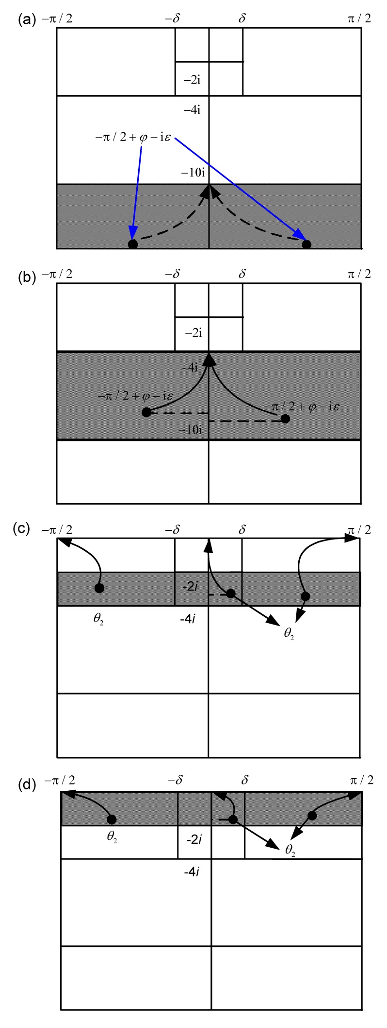
For this numerical simulation within the domain [−π/2, θ2], we divide the complex θ-plane into regions as shown in Fig. 6, which is proposed by Iwashita (1997). We consider a different treatment of the integration path for each case, and choose different integration methods. In Fig. 6, δ is a relatively small value and set as δ=π/16 in actual calculation.
(a) For the condition of ε≥10 including the case of X=Y=0
The integrand tends to zero as ε tends to infinite. We can therefore neglect the integration from θ2 to −10i as the order of the integrand is less than O(10−8) in the magnitude at θ2=−10i. The integration path is taken as straight lines shown in Fig. 6a, because the steepest descent line from, i.e., θ=−10i is regarded as the imaginary axis and the real axis towards θ=−π/2. At this point, we calculate the integration along the real axis by the VSM, which is different from Iwashita (1997)’s method and proved to be efficient.
(b) For the condition of 4≤ε<10
The path from θ2 is taken to be close to the imaginary axis by using the B-spline discussed by Yao and Dong (2013). The cross points between the dotted line and the imaginary axis are used for the control points of the B-spline. Here, the integration along the real axis is also calculated by the VSM to avoid the complication of numerical search of the steepest descent line when the start point is located on the real axis.
(c) For the condition of 2≤ε<4
If Re(θ2)≤−π/16, the path is toward θ=−π/2; otherwise, if Re(θ2)≥π/16, the path is toward θ=π/2; meanwhile, if −π/16θ
2)<π/16, an approximate integral path is taken, which is similar to Clause (b).
(d) For the condition of 0≤ε<2
When the starting point θ2 is located in this region, the numerical search of the steepest descent line becomes necessary near θ=±π/2. However, when −δθ
2)<δ, an approximate integral path is taken too, which is similar to Clause (c).
Fig.6 Arrangement of the integral path: (a) ε≥10; (b) 4≤ε<10; (c) 2≤ε<4; (d) 0≤ε<2
The numerical search algorithm of the steepest descent line has been discussed by Iwashita and Ohkusu (1989) and Du and Wu (1998). When |Z| and |Y| are close to zero compared to |X|, then the integrands of Eq. (2a) are so large at the start point and decrease too rapidly for numerical integration to be appropriate. For this case, a complementary scheme should be introduced as illustrated in (Iwashita and Ohkusu, 1989; 1992; Du, 1996; Du and Wu, 1998).
4.4. Self-adaptive integration method in parametric domain
The self-adaptive integration method to calculate the integral along the steepest descent line was firstly established by Du (1996) to evaluate translating-pulsating Green’s function in Bessho form. To improve the efficiency of this method, some modifications are introduced as follows.
1. The steepest descent line generally forms a curved line of sometimes small curvature, so this line can be represented by a typical B-spline curve. The knots vectors are established via accumulative chord length method so as to acquire a parameter interval [0, 1]. The discrete points on the steepest descent line are represented by the B-spline, which is expressed by
,
where is a set of control points coinciding with the coordinate of the steepest descent line. is the basis function of the B-spline, which can be defined as follows:
,
where ui is a knot value, is a knot vector. The accumulative chord length method is discussed as follows.
If is a discrete point on the steepest descent line, S is the total length of this line, s is the total number of discrete points, then:
,
When the steepest descent line is represented by the B-spline curve, one-one correspondence exists between discrete points and parameter t, where t∈[0, 1].
2. As in the self-adaptive algorithm, we first subdivide the entire integral domain of t into several equal segments and treat each part separately. The length of each segment is 1/l and the total integral is the sum of them. Here, the high order trapezoidal integration rule is used and, if necessary, repeatedly subdivides the range automatically. Details are listed by Du (1996) and Du and Wu (1998).
.
The self-adaptive integration method presented here is an integral method performed one time along the steepest descent line represented by the B-Spline curve. The refined integration points are just on the B-spline curve, without any discretization of the integration relating to the discrete path. This avoids the waste of CPU time for numerical search of the refined points on the steepest descent line as obtained by Du and Wu (1998).
4.5. Truncation of numerical integration
If , the integrands tend to zero, so we truncate the numerical integration somewhere on the integral path for high efficiency. It can be known from (Du, 1996) that the truncation error is lower than 10−5 when choosing a truncation point at . The finite upper limit of the integral is calculated by Eqs. (23a) and (23b) when θ is on the real axis.
,
5. Numerical results and analysis
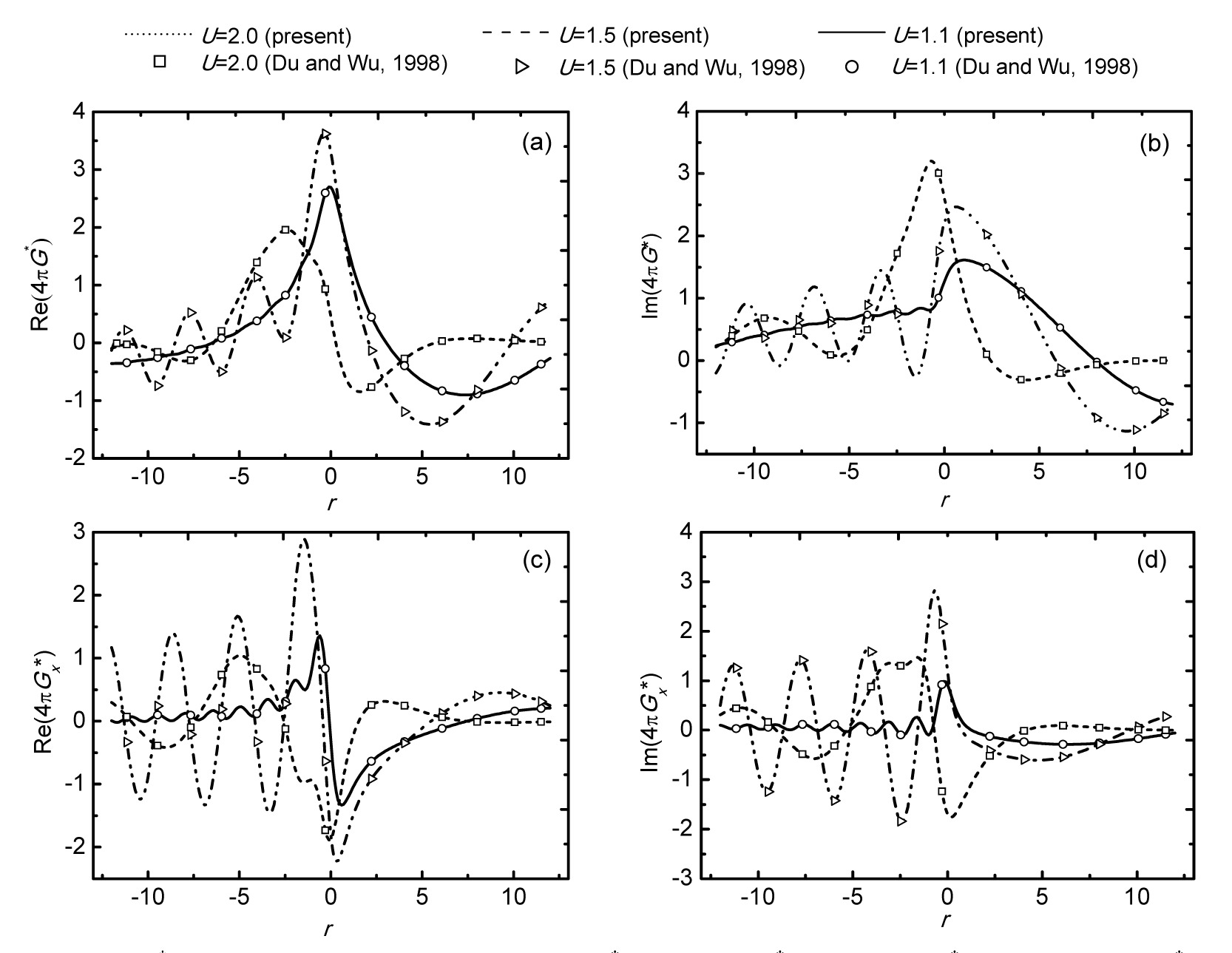
To check the effectiveness of the proposed numerical integration methods, curves G* and Gx* are plotted in Fig. 7 and Fig. 8. The same cases have been presented by Du and Wu (1998) and Du et al. (2005). The calculated conditions for Fig. 7 are ωe=1.4 rad/s, and U=1.1 m/s, 1.5 m/s, and 2.0 m/s. Fig. 8 shows that the source point is located at (0, 0, 0), and the field points describe the x-axis, corresponding to Y=0. The excellent level of agreement with known results shows that the present numerical method is reliable.
Fig.7 Images of G* and its partial derivative for Re(4πG*) (a), Im(4πG*) (b), Re(4πGx*) (c), and Im(4πGx*) (d)
Fig.8 Images of G* and its partial derivative for Re(4πG*) (a) and Re(4πGx*) (b)
The total average CPU time consumed to calculate G* and its partial derivatives is scattered from 4×10⁻³ s to 6×10⁻³ s, meeting the requirements of engineering applications.
6. Conclusions
In this paper, the performance of Bessho form translating-pulsating source Green’s function is discussed and a numerical integration method is proposed. Conclusions can be drawn as follows.
θ1 is an infinite jump discontinuous node and can be eliminated by use of the Gaussian quadrature rule. For this rule, the end points of the integration interval must satisfy .
The performances of H1 and H2 are influenced by ρ and Z. As for H2, only when the parameter ρ is very large and the value of |Z| is small, can H2 act as high-frequency oscillatory; H1 becomes high-frequency oscillatory not only when ρ is very large but also when θ→−π/2. However, H1 attenuates very fast when θ approaches −π/2 since |k1Z| is also very large and H1 becomes zero when θ→−π/2. To efficiently evaluate these terms, the combination of SDIM in the θ-plane and VSM can be adopted.
Numerical results have proved the efficiency and accuracy of present method, and it can be further developed to calculate the diffraction-radiation problems of floating structures advancing in waves.
Acknowledgements
The authors would like to thank Prof. Gerard DELHOMMEAU from Laboratoire de Mecanique des Fluides, Ecole Centrale, France, and Prof. Hidetsugu IWASHITA from Department of Energy and Environmental Engineering, Faculty of Engineering, Hiroshima University, Japan for the evaluation discussion on the Green’s function.
[1] Abramowitz, M., Stegun, I.A., 1964. Handbook of Mathematical Functions. Dover Publications,New York :
[2] Bailey, P.A., Hudson, D.A., Price, W.G., 2001. Comparisons between theory and experiment in a seakeeping validation study. Transactions of the Royal Institution of Naval Architects, 143:44-77.
[3] Bessho, M., 1977. On the fundamental singularity in the theory of ship motion in a seaway. Memoirs of the Defense Academy Japan, 18(3):95-105.
[4] Brument, A., Delhommeau, G., 1997. Evaluation numerique de la function de Green de la tenue a la mer avec vitesse d’a vance. Journees de Lhydrodynamique, (in French),25:147-160.
[5] Chen, X.B., Wu, G.X., 2001. On the singular and highly oscillatory properties of the Green function for ship motions. Journal of Fluid Mechanics, 445(1):77-91.
[6] Du, S.X., 1996. A Complete Frequency Domain Analysis Method of Linear Three-dimensional Hydro-elastic Responses of Floating Structures Travelling in Waves. PhD Thesis, (in Chinese), China Ship Scientific Research Center,Wuxi, China :
[7] Du, S.X., Wu, Y.S., 1998. A fast evaluation method for Bessho form translating-pulsating source Green’s function. Shipbuilding of China, (in Chinese),2:40-48.
[8] Du, S.X., Hudson, D.A., Price, W.G., 2005. Prediction of three-dimensional seakeeping characteristics of fast hull forms: influence of the line integral terms. , International Conference on Fast Sea Transportation, Petersburg, Russia, 1-8. :1-8.
[9] Du, S.X., Hudson, D.A., Price, W.G., 2012. An investigation into irregular frequencies in hydrodynamic analysis of vessels with a zero or forward speed. Journal of Engineering for the Maritime Environment, 226(2):83-102.
[10] Fang, M.C., Chan, H.S., 2002. Numerical study of hydrodynamic pressure on a high speed displacement ship in oblique waves. Bulletin of the College of Engineering, NTU, 86:15-22.
[11] Haskind, M.D., 1953. The hydrodynamic theory of ship oscillations in rolling and pitching. Technical Research Bulletin, 1(12):45-60.
[12] Iwashita, H., 1997. An improvement computation method of the seakeeping Green function. Technical Report, the University of Hamburg,:
[13] Iwashita, H., Ohkusu, M., 1989. Hydrodynamic forces on a ship moving with forward speed in waves. Journal of Society of Naval Architects of Japan, (in Japanese),166:187-205.
[14] Iwashita, H., Ohkusu, M., 1992. The Green function method for ship motions at forward speed. Ship Technology Research, 39:3-21.
[15] Maury, C., 2001. Etude du Problem de la Tenue a la Mer Avec Vitesse Davance Quelconque par une Method de Singularites de Kelvin. PhD Thesis, (in French), Laboratoire de Mecanique des Fluids,Nantes, France :
[16] Maury, C., Delhommeau, G., Ba, M., 2003. Comparison between numerical computations and experiments for seakeeping on ship models with forward speed. Journal of Ship Research, 47:347-364.
[17] Miao, G.P., Liu, Y.Z., Yang, Q.Z., 1995. On the 3-D pulsating source of Michell’s type with forward speed. Shipbuilding of China, (in Chinese),4:1-11.
[18] Rahman, M., 1990. Three dimensional Green’s function for ship motion at forward speed. International Journal of Mathematics and Mathematical Sciences, 13(3):579-590.
[19] Xu, Y., Dong, W.C., 2011. A fast integration method and characteristics research for 3-D translating-pulsating Green’s function of Havelock form in deep water. China Ocean Engineering, 25(3):365-380.
[20] Yao, C.B., Dong, W.C., 2013. Study on fast integration method for Bessho form translating-pulsating source Green’s function. Technical Report 2013051. (in Chinese), Naval University of Engineering,China :
[21] Zakaria, N.M.G., 2006. A Design Aspect on the Seakeeping Performances of Ships by 3-D Greens Function Method with Forward Speed. PhD Thesis, Yokohama National University,Yokohama, Japan :
[22] Zakaria, N.M.G., 2009. Effect of ship size, forward speed and wave direction on relative wave height of container ships in rough seas. The Journal of the Institution of Engineers, 72(3):21-34.
[23] Zong, Z., Qian, K., 2012. A three-dimensional moving and pulsating source method for calculating motions of trimaran hull forms. Journal of Ship Mechanics, (in Chinese),16(11):1239-1247.
Open peer comments: Debate/Discuss/Question/Opinion


Open peer comments: Debate/Discuss/Question/Opinion
<1>