Similar articles

Abstract: Traditional crash frequency modeling uses crash frequency data averaged across multiple years. When data size is small, crash data in each year are used in the modeling to extend the size of the samples. The extension of sample size could create a temporal correlation among crash frequencies of the different years, which could affect the modeling accuracy. The primary objective of this study is to evaluate the application of the generalized estimating equation (GEE) procedures to account for the temporal correlation in the longitudinal crash frequency data. Four-year crash data at exit ramps on a freeway in China were collected for modeling. Based on the same data, traditional generalized linear models (GLMs) were estimated for model comparison. Results showed that traditional GLM underestimated the standard errors of coefficients for explanatory variables. The GEE procedure with an exchangeable correlation structure successively captured the temporal correlation among the crash frequencies of the different years. The GLM with GEE outperformed the traditional GLM in providing a good fit for the crash frequency data. Results of this study can help researchers better understand how various factors affect the crash frequencies at freeway divergent areas and propose effective countermeasures.

基于广义估计方程的时间相关性事故频次建模

研究目的：采用广义估计方程模型对存在时间相关性的事故频次数据进行建模，并与传统广义线性模型的估计效果进行对比。
创新要点：通过广义估计方程来考虑事故频次建模中数据的时间相关性，从而提高参数估计准确度以及模型预测精度。
研究方法：基于4年高速公路交通事故频次数据，建立考虑时间相关性的广义估计方程以及传统的广义线性模型，并采用统计指标对模型效果进行对比。
重要结论：1.事故频次数据样本量对预测精度影响很大；2.广义估计方程能够有效考虑事故频次数据中存在的时间相关性；3.广义估计方程的参数估计比传统广义线性模型更准确，且精度更高。

关键词：广义估计方程；事故频次；时间相关；广义线型模型

1.  Introduction

 Road infrastructure and traffic volume have dramatically increased over the past decades in many countries, resulting in a considerable increase in traffic crashes (Saenghaengtham and Kanongchaiyos, 2006; Hu et al., 2008; Jin et al., 2011; Luoma and Sivak, 2012; Li et al., 2012; 2013; 2014; Ma et al., 2012; Jin et al., 2013). An analysis on crash frequency can identify factors that affect the crashes to help reduce the number of crashes. Previously, numerous crash prediction models have been developed. Various methodologies have been proposed for crash frequency modeling to improve the predictive accuracy for crashes (Lord and Mannering, 2010).

 In most of the previous crash prediction models, crash counts were usually aggregated over several years and the average crash count per year was considered the response variable (Bauer and Harwood, 1998; Bared et al., 1999; McCartt et al., 2004; Chen et al., 2009; 2011; Lord and Mannering, 2010; Liu et al., 2010; Washington et al., 2010). The reason for this is to reduce the random variation in the yearly crash data. The maximum likelihood estimation (MLE) method is used to estimate the coefficient and significance level of each predicting factor in the model. The MLE method can produce accurate model estimates when the dataset contains a large number of recordings.

 However, researchers or agencies in many countries, especially in developing countries, are often faced with the small sample size issue in the crash data. Due to the restrictions on the crash reporting systems, there is usually no gateway for the public to access the resources of crash recordings as well as road and traffic information. Moreover, important information is often missing in the original dataset which further reduces the sample size that is useful for modeling. With the data of a small sample size, the desirable properties of some parameter-estimation techniques, such as the MLE, are not realized (Washington et al., 2010). Biased estimates and incorrect inferences could occur in the crash prediction models.

 To enlarge the sample size in the dataset, a natural consideration is to divide the data aggregated over several years into smaller time intervals (a unit of year) and treat the crash counts in each year as separate observations. The enlarged sample size would improve the estimating accuracy of the crash prediction model. However, disaggregating the crash data could create a temporal correlation in the dataset. Crash counts in different years could be correlated with each other due to the unobserved or unconsidered effects of factors associated with a specific road entity that do not change over years. This fact becomes rather determinate in developing countries since the information of important factors is often missing. The temporal correlation could adversely affect the precision of parameter estimates in the crash prediction model if not properly considered in the modeling procedure (Lord and Persaud, 2000).

 Previously, safety researchers have proposed numerous sophisticated methodologies to account for the correlations among groups of crash frequencies. Those methodologies include the generalized estimating equation (GEE) (Lord and Persaud, 2000; Wang and Abdel-Aty, 2006; 2008), the random-effects model (Shankar et al., 1998; Miaou and Lord, 2003; Quddus, 2008), the hierarchica/multilevel model (Jones and Jørgensen, 2003; Kim et al., 2007), and the multivariate modeling approaches (Ma and Kockelman, 2006; Park and Lord, 2007; El-Basyouny and Sayed, 2009). However, several models may not be appropriate for practical applications because they are very complicated and difficult to solve. The safety researchers or agencies often experience great difficulties in trying to select the appropriate method for their particular needs.

 In this study, the main objective is to evaluate the application of GEEs to account for the temporal correlation in the crash frequency modeling. To achieve the research objective, four-year crash data were collected from exit ramps on a freeway in China. Procedures of traditional generalized linear models (GLMs) as well as a GLM with GEE were estimated for model comparison. The findings of this study can provide useful information to researchers in developing crash prediction models based on the crash frequency data with temporal correlations.

2.  Data

 The data were collected from 32 sections of exit ramps on the Guangshen freeway in China. The freeway has a total length of 98 km and is located in the southern part of China. The freeway connects several of the most economically developed cities in Guangdong province and there is a high traffic demand on both the mainline and ramps. Traffic crashes frequently occur at the exit ramp areas on this freeway.

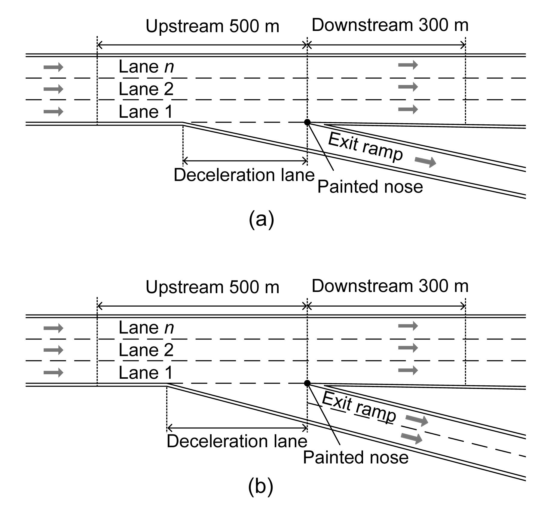
 In this study, the exit ramp areas include two sub-segments that are located in the upstream and downstream of the painted nose. In previous studies, a section with 457.5 m (1500 ft) in the upstream and 304.8 m (1000 ft) in the downstream was considered as the influencing area of an exit ramp (Chen et al., 2009; Liu et al., 2010). On the Guangshen freeway, the message signs for exits are usually posted 500 m upstream of the exits. Thus, a section with 500 m in the upstream and 300 m in the downstream of the painted nose is considered as the exit ramp area. The illustration of exit ramp areas is shown in Fig. 1.




 Local freeway agency would like to identify which factors are related to the number of crashes to evaluate the safety performance of exit ramps. They want to identify the ramps that have higher than normal crashes and implement countermeasures to reduce the crashes. To reach their objective, a large dataset is usually required to obtain accurate estimates on the safety impacts of explanatory factors (Hauer, 1997). However, it is difficult to obtain crash data as well as road and traffic information on other neighboring freeways since this information is not shared. Only the data from 32 exit ramps on the freeway are available.

 Four-year crash data, from 2006 to 2009, were obtained from the local freeway management agency. A total of 4429 crashes were observed. The crashes included all types of injury severities. The statistics of the crash counts are shown in Table 1. The average crash count per year is 34.60 with a standard deviation (SD) of 38.87. The crash data have an obvious feature of over-dispersion since their mean values are much smaller than the variance.




 There are two types of exit ramps that are typical on the Guangshen freeway, according to the number of exit lanes shown in Fig. 1. The road geometric attributes, such as the number of lanes, presence of longitudinal grade, and right shoulder width, are identified from the design drawing manual of the freeway. The speed limit information and average daily traffic of the mainline and exit ramps were obtained from the freeway management company. The percentage of days with severe weather in each year was also obtained from recordings. The summary statistics of these explanatory variables are shown in Table 2.

3.  Hardware and embedded safe operation system (ES-OS)

 This section briefly describes the traditional GLM for crash frequency modeling and the GEE procedure to account for the temporal correlation in longitudinal data. The cumulative residual test and type III analysis for model assessment are also introduced.

3.1.  GLM for crash frequency analysis

 When applying the GLM for crash frequency analysis, the random component is often likely to follow a Poisson or negative binomial (NB) distribution (Washington et al., 2010). After reviewing the model specifications for crash frequency analysis at freeway exit ramps in (Lord and Mannering, 2010), the following model form is considered: (1) , where ln(E{μ_t }) is the natural log of expected crash frequency in period t at the exit ramps, u_t is the crash frequency in period t, F ₁(t) and F ₂(t) are annual average daily traffic (AADT) on the mainline and ramps in period t, respectively, X_j (t) is the jth explanatory variable in period t, and β_j is the jth coefficient to be estimated (j=0, 1, …, J), J is the number of coefficient of variables. The average crash frequency per year across the four years was used in the GLM when t was set to 1 year. To enlarge the sample size, the crash frequency data could be disaggregated by a small time interval, which is one year at each ramp. Thus, the model based on yearly aggregated data is determined when t was set to 4 year.

3.2.  GLM with GEE procedure

 In the model based on yearly disaggregated data in Eq. (1), the crash frequency in a year could be correlated with others. The GEE is an extension of the GLM for estimating the temporally correlated data. Using the link function shown in Eq. (1), the coefficients β are estimated by (Lord and Persaud, 2000) (2) , where D _i is the J×T matrix of partial derivatives of the mean with respect to the regression parameters, T is the number of years, u _i is the predicted crash count at the ith ramp, I is the number of ramp, i indicates the ith ramp, Y _i is the observed crash frequency at the ith ramp, and V _i is the covariance matrix defined as (3) , where A _i is a T×T diagonal matrix with V(μ_it ) as the tth diagonal element, R _i ( λ ) is the T×T matrix presenting the temporal correlation in repeated observations, and λ is the type of correlation with λ =[λ ₁, λ ₂, …, λ_{n −1}] and λ_i =cor(Y_t , Y_k ) for t, k=1, 2, …, n−1, t≠k.

 To solve the model with GEE correctly, every element of the correlation matrix R _i has to be known. However, in many instances, it is not possible to know the proper correlation type for the crash counts per year. To overcome this drawback, Liang and Zeger (1986) proposed a “working” matrix as the correlation matrix to estimate the coefficients. The commonly used correlation structure in the GEE procedure is briefly described as follows:

1. Independent: the independent correlation structure assumes that repeated observations (crash counts in different years) for an exit ramp are independent. In this case, the GEE estimates are the same as the regular GLM in the coefficients but different in the standard errors (SEs).

2. Exchangeable: the exchangeable working correlation assumes constant correlations between any two observations within an exit ramp.

3. Autoregressive: the autoregressive correlation structure weighs the correlation between two observations by their separated time-gap (order of measure). As the gap distance increases, the correlation decreases.

4. Unstructured: the unstructured correlation structure assumes a different correlation between any two observations taken at the same location.

3.3.  Model assessment

 Traditional goodness-of-fit tests for basic GLM are not valid for the GLM with GEE procedure (Wang and Abdel-Aty, 2006). The cumulative residual tests are conducted to graphically and numerically examine how well the link function fits the dataset. The cumulative residual method has an advantage of being independent on the number of observations as are many other traditional statistical procedures (Hauer, 2004; Wang and Abdel-Aty, 2006; 2008). If the model is correct, the residuals should be centered at zero and the plot of the residuals against any coordinate should exhibit no systematic tendency. The maximum absolute value of the observed cumulative sum and the P-value for a Kolmogorov-type supremum test are calculated. A small maximum absolute value and a large P-value indicate a better model performance.

 The type III analysis has been used to identify a variable’s relative significance (Wang and Abdel-Aty, 2006; 2008). The type III χ² value for a particular variable is the difference between the generalized score statistic or likelihood ratio statistic for the model with all the variables included and that with this variable excluded. A small P-value indicates that the effect of this variable is highly significant.

4.  Results

 The crash data in this study are shown to be over-dispersed so that the GLM with a NB distribution in the random component is considered to fit the data. Two traditional GLMs based on yearly aggregated and disaggregated crash data are evaluated and a GLM with GEE procedure is fitted. The model estimates are compared and the results are discussed.

4.1.  GLM model estimates

 Two GLMs are estimated in this section: the first model (GLM 1) uses the average crash count per year across the four years as the dependent variable; and the second model (GLM 2) uses the crash count in each year. The GLMs take the model forms in Eq. (1) and the explanatory variables are carefully selected to determine the final model specifications. The estimates of the two GLMs are shown in Table 3. Only the variables that are significant in at least one model are included.




 In the GLM 2, five variables are significantly related to the crash count per year at a 90% confidence level. These variables include the AADT on mainline, AADT on exit ramp, presence of grade, bad weather ratio, and right shoulder width. However, in the GLM 1, only two variables, the bad weather ratio and right shoulder width, are estimated to be significant at a 90% confidence level. The other variables such as AADTs on mainline and ramp are not statistically significant, which is contrary to the intuition. The performance of the GLM 1 would attribute to the impact of a small sample size in the dataset. This is supported by the fact that the GLM 2 has a better statistical fitness than the GLM 1 as shown in Table 3. These results show how the small sample size issue impacts the model estimates and leads to poor model performances.

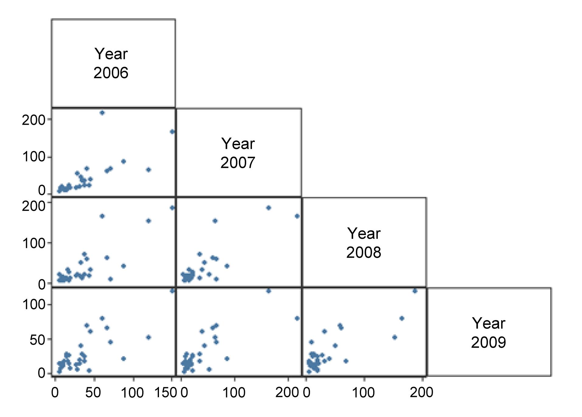
 Traditional GLMs assume that the response variable (crash count in this study) is independent of each other, which may not be true for the longitudinal data with repeated observations over time at each location. Crashes in different years could be intercorrelated due to the unobserved or unconsidered effects of factors associated with a specific exit ramp that did not change over the years. Fig. 2 shows that the correlation exists between crashes of different years. The traditional GLM with yearly disaggregated data developed above did not account for the temporal correlation in the dataset and could result in biased model estimates.

4.2.  Model estimates with GEE

 The GLM model with GEE procedure is fitted using the yearly disaggregated data to account for the temporal correlation. Four types of correlation structure, which are the independent, exchangeable, autoregressive, and unstructured structure, are explored in the GEE procedure. The estimating results of these models are shown in Table 4. It can be identified that the coefficients and SEs for explanatory variables are consistent between models with different correlation structures. It indicates that the GEE approach has a robust performance and that the estimates would be correct even when the covariance matrix is specified incorrectly (Lord and Persaud, 2000). Though the estimates are similar, the four models produce unequal estimating results, which shows the impacts of different correlation structures in the GEE procedure.




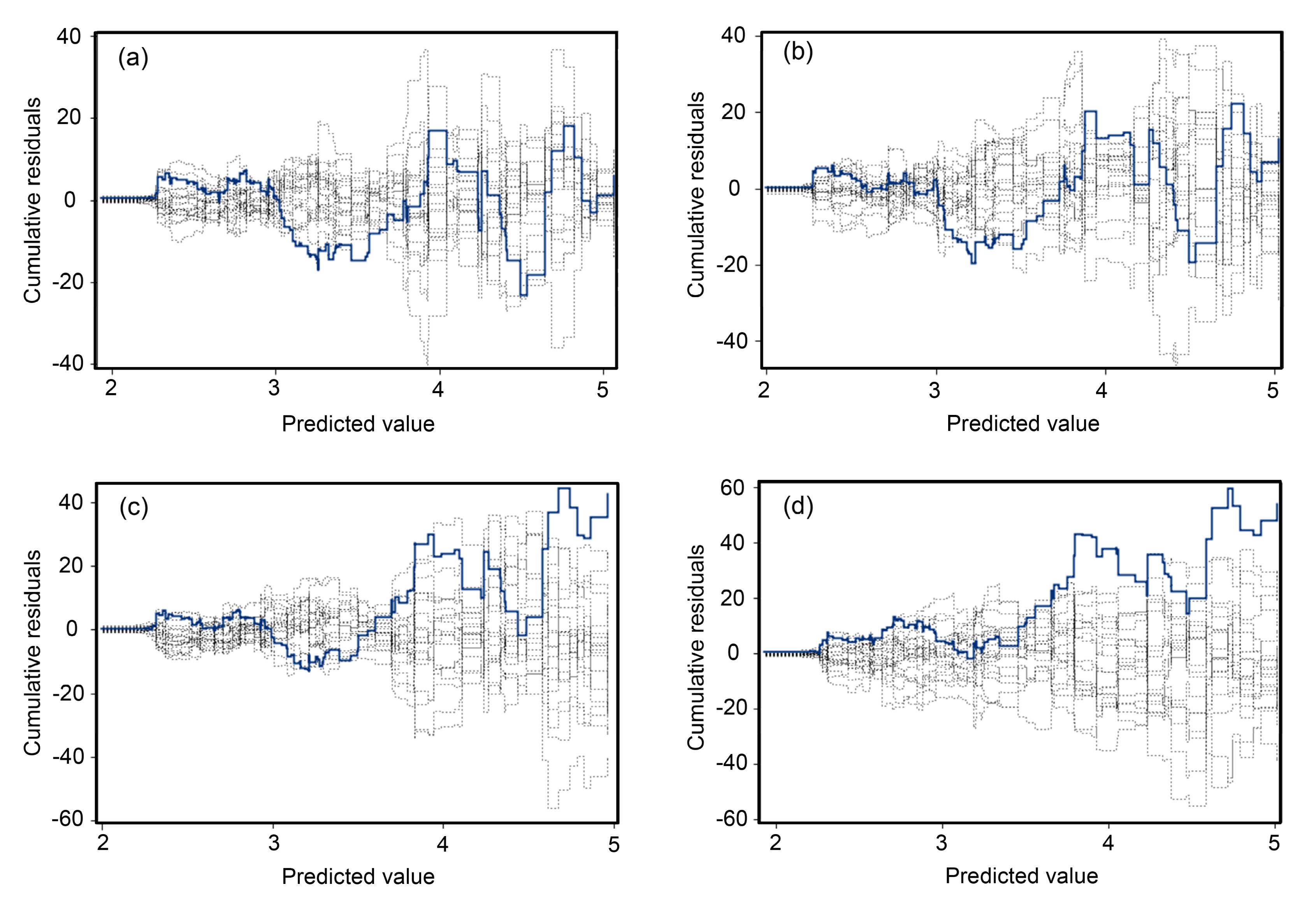
 The estimated correlation matrix with a dimension of four for each type of correlation structure is shown in Table 5. The assessments of models with different correlation structures are performed using the cumulative residual test, and the results are shown in Fig. 3. The observed cumulative residuals for working correlation structures are represented by the heavy lines, and the simulated curves are represented by the light lines. The residuals for the GEE with exchangeable correlation structures are centered at zero and the plot of the residuals against any coordinate exhibits no systematic tendency. Also as shown in Table 4, the GEE with exchangeable structure has the smallest maximum absolute value and the largest P-value among all the structures. These assessments indicate that the exchangeable structure in the GEE is fairly appropriate to fit the inherent feature of data in this study.







 The exchangeable structure assumes that the correlations between multiple observations are constant. As shown in Table 5, the correlation between two successive observations is 0.271, indicating that there is a significant temporal correlation between crash counts at an exit ramp in different years. The relatively high correlation should not be neglected during the crash modeling procedure. In some previous studies, the autoregressive structure in GEE was found to have the best goodness-of-fit since it assumed that the correlation between observations would decrease as the time-gap increases (Wang and Abdel-Aty, 2006). The different findings on the performance of correlation structure between this study and previous ones would be explained by the different characteristics of crash data that have been used. In this study, it is identified that the exchangeable correlation structure is more consistent than the correlation plots shown in Fig. 2.

 In sum, with the results obtained above, it is reasonable to conclude that: (1) there is obvious temporal correlation in the crash data with yearly disaggregated observations; (2) the exchangeable working correlation structure is the most fitted one in the GEE procedure for analyzing the four-year frame data in this study.

4.3.  Comparison between models

 A comparison on the coefficient and SE of each variable between the GLM 2 and the GLM with GEE shows that though the coefficients are shown to be similar in the two models, the SEs in the GLM with GEE are obviously larger than those in the traditional GLM 2. This result suggests that the temporal correlation contributes to a large amount of SEs for explanatory variables. The increase of SE would decrease the significant level of a variable. In other words, some factors may become insignificant after considering the temporal correlation in the data.

 Recall that the temporal correlation in the crash data is generally generated by the unobserved or unconsidered effects of factors that do not change over years on an exit ramp. If the temporal correlation is not properly considered in the modeling procedure, the variation of crash counts could be incorrectly attributable to the variation of observed variables, other than these unobserved effects. In the traditional GLM, the estimated effects of explanatory variables potentially contain some effects of unobserved factors. In this situation, the inferences on the impacts of contributing variables on crashes could still be biased and misleading.

 The type III analyses are performed to examine the relative significance of explanatory variables. As shown in Table 6, the type III χ² values in the GLM with GEE are generally smaller than that in the GLM 2 and the P-values for variables are larger in the GLM with GEE. It indicates that the traditional GLM without accounting for the temporal correlation would overestimate the significance of predicting factors, which is consistent with previous studies (Lord and Persaud, 2000; Wang and Abdel-Aty, 2006; 2008).




 As shown in Table 6, the right shoulder width is estimated to be significantly related to crash counts at a 90% confidence level in the GLM 2. However, after considering the temporal correlation in the GLM with GEE, this variable becomes insignificant at the same confidence level. Though more crashes are reported at exit ramps with narrower right shoulders, the large number of crashes would be due to some effects of unobserved factors such as poor pavement or unsafe geometric designs (which are reflected in the temporal correlation) other than the effect of the right shoulder width. If the shoulder width was incorrectly considered to predict the normal safety level for exit ramps, some true hotspots with higher-than-normal crashes could not be identified correctly. Considering the temporal correlation using the GEE procedure could result in more accurate inferences. It could help safety researchers or agencies make correct decisions to implement countermeasures on dangerous ramps.

4.4.  Interpretation of coefficients

 The AADTs on mainline and ramps are estimated to be positively related to crash counts at exit ramps. The increase of traffic volume results in an increase of traffic crashes. The coefficient for AADT on ramp is larger than that for AADT on mainline suggesting that a unit increase in traffic volume on an exit ramp could generate more crashes as compared to that on a mainline. The presence of grade will increase the crash counts since the estimated coefficient for the variable is positive. More crashes are likely to occur under bad weather conditions.

 Several insignificant explanatory variables were reported to be significant predictors in some studies. For example, the length of the deceleration lane and the length of the exit ramp have been identified to be significantly related to crash counts at freeway exit ramp areas (Chen et al., 2009; 2011; Liu et al., 2010). It could be difficult to tell if the insignificances of these variables in this study reflect the actual situation on the freeways in China or are generated due to the limitation of sample size used for model development. These variables at a ramp do not vary over years so that the disaggregation of data per year could not improve the estimates for these variables. Data with larger sample size are always desirable to obtain more accurate estimates on the relationships between these variables and crash counts.

5.  Conclusions and discussion

 This study evaluated the application of the GEE to account for the temporal correlation in the crash frequency data. Using four-year crash data at exit ramps on the Guangshen freeway, China, the GLM with GEE was estimated based on yearly disaggregated crash data. For comparison purposes, traditional GLMs were also estimated based on the same dataset.

 The results showed that there were significant temporal correlations in the yearly disaggregated crash data used in this study. The GEE procedure captured the correlation among crash counts in different years. The exchangeable correlation structure fitted the data properly. A comparison between the GLM and the GLM with GEE showed that the traditional GLM could underestimate the SEs of explanatory variables and make incorrect inferences on the significance of the variables. The GLM with GEE captured the features of temporal correlation in the data and led to more accurate estimates on the impacts of predictors. In the modeling results, the right shoulder width was identified to be a significant factor in the traditional GLM, but became insignificant after accounting for the temporal correlation in the GLM with GEE. Other contributing factors on crashes at freeway exit ramps included the AADT on mainline, AADT on ramps, presence of grade, and bad weather ratio.

 The findings of this study suggest that the GEE is an appropriate approach for modeling crash frequency data with temporal correlation. This approach makes it relatively easy to develop proper and accurate crash prediction models even if the type of temporal correlation is unknown. The GEE procedure also has an advantage that many statistical software packages already have a built-in GEE functionality.

 Even though this study showed that using disaggregated crash data results in better model predictions than using aggregated crash data, such a conclusion does not hold true in many situations. This study simply showed that the models with enlarged sample size (by extending data to more than one year) perform better than the models with small sample size. However, it does not mean that the models based on monthly or weekly crash data will definitely outperform those with yearly crash data, because the predicted values of the models are rather different. Detailed experiments and modeling are required to compare the performances of different models based on different temporal segmentations of crash data. Besides, it should be explained that extending the crash data to smaller aggregation intervals may lead to an increase in the number of sections with zero counts, leading possibly to the need for zero-inflated models, since excessive zero counts do not fit the regular Poisson or negative binomial models.

 The observations from the same year may be correlated due to unobserved within-year effects, which are termed as the spatial correlation. Though the GEE procedure can successfully account for the temporal correlation in the crash frequency data, it cannot address the spatial correlation that could also exist in the crash data. Recently, researchers have proposed more sophisticated models which can account for the spatial correlation across locations, such as the random-effects model (Shankar et al., 1998; Miaou and Lord, 2003; Quddus, 2008) and the hierarchica/multilevel model (Jones and Jørgensen, 2003; Kim et al., 2007). Considering the spatial correlation in the modeling procedure could improve the model predictions. The authors recommend that future studies could focus on these issues.

---

* Project supported by the National Key Basic Research Program (973) of China (No. 2012CB725400), the National High-Tech R&D Program (863) of China (No. 2012AA112304), and the National Natural Science Foundation of China (No. 51338003)