Bin He, Xin-biao Xiao, Qiang Zhou, Zhi-hui Li, Xue-song Jin. Investigation into external noise of a high-speed train at different speeds[J]. Journal of Zhejiang University Science A, 2014, 15(12): 1019-1033.
@article{title="Investigation into external noise of a high-speed train at different speeds", author="Bin He, Xin-biao Xiao, Qiang Zhou, Zhi-hui Li, Xue-song Jin", journal="Journal of Zhejiang University Science A", volume="15", number="12", pages="1019-1033", year="2014", publisher="Zhejiang University Press & Springer", doi="10.1631/jzus.A1400307" }
%0 Journal Article %T Investigation into external noise of a high-speed train at different speeds %A Bin He %A Xin-biao Xiao %A Qiang Zhou %A Zhi-hui Li %A Xue-song Jin %J Journal of Zhejiang University SCIENCE A %V 15 %N 12 %P 1019-1033 %@ 1673-565X %D 2014 %I Zhejiang University Press & Springer %DOI 10.1631/jzus.A1400307
TY - JOUR T1 - Investigation into external noise of a high-speed train at different speeds A1 - Bin He A1 - Xin-biao Xiao A1 - Qiang Zhou A1 - Zhi-hui Li A1 - Xue-song Jin J0 - Journal of Zhejiang University Science A VL - 15 IS - 12 SP - 1019 EP - 1033 %@ 1673-565X Y1 - 2014 PB - Zhejiang University Press & Springer ER - DOI - 10.1631/jzus.A1400307
Abstract: This paper presents a detailed discussion of the experimental analysis of the external noise produced by a Chinese high-speed train traveling at different speeds. Based on the delay and sum beam-forming method, a microphone array with 78 microphones was used to measure the external noise produced by the train moving at speeds of up to 390 km/h. The experiment and its analysis showed that the main noise produced by the train originates in three areas: the wheel/rail system (or bogies), the pantograph, and the inter-coach gaps of the train. The frequency characteristics and sound exposure level (SEL) of these main sources were analyzed for different speeds. In the range of 5000 Hz, the SELs of the three main noise sources are clearly identified. Along the vertical height of the train, as seen from the rail head, the maximum noise levels always occur in the wheel/rail area. At different measurement field points, the predominant noise components of the total noise have different frequencies that vary with the train speed. Furthermore, at the measurement points, the rolling noise has a greater contribution to the total noise than the aerodynamic noise. The experimental results and their corresponding analysis are very useful for the control and reduction of the external noise produced by high-speed trains.
Darkslateblue:Affiliate; Royal Blue:Author; Turquoise:Article
Article Content
1. Introduction
The noise generated by high-speed trains is a sensitive issue, as high-speed train tracks are built in densely populated areas, where prior noise levels were very low. There is a need for an accurate description of the main characteristics (position, strength, spectrum, energy contribution, etc.) of different noise sources of moving high-speed trains, since this information is typically used as input for noise prediction and to guide studies on noise mitigation measures.
Over the past decades, many studies have been performed to determine the noise sources of high-speed trains and their precise characteristics. It has been recognized that the main noise sources are rolling noise, aerodynamic noise, and traction noise (Thompson, 2008). However, so far it has been difficult to clearly distinguish the location of these noise sources and their independent contribution to the total noise of a traveling high-speed train. In this respect, the beam-forming method is able to effectively identify individual noise sources. As a signal processing technique, this method has been used in microphone arrays for signal transmission and reception (Christensen and Hald, 2004). Recently, Dittrich and Janssens (2000) developed a T-like microphone array to identify the noise sources of trains. Based on near-field acoustical holography, Schulte-Werning et al. (2003) developed a spiral-like microphone array with a diameter of 4.0 m. Within the Deutsche Bahn ‘low-noise railway’ project, noise sources from ICE high-speed trains were recognized in a frequency range of 200–3150 Hz. Furthermore, noise source identification experiments on TGV trains moving at speeds from 250 km/h to 320 km/h were carried out, and the distribution of aerodynamic and wheel/rail rolling noise was analyzed (Mellet et al., 2006). Silence (2005) carried out source identification for TFS tramcars and a CITADIS 302 train for traveling speeds of 20 km/h to 100 km/h, and reported that wheel/rail noise was the major noise source, and 5.0–10.0 dB(A) larger than other noise sources. The spiral-like microphone array was also used for the Japanese Shinkansen train and for noise source identification tests of Fastech 360S trains (Wakabayashi et al., 2008). When the speed of the trains reached 340 km/h, the maximum noise came from their wheels. Poisson et al. (2008) carried out noise source identification for TGV trains and arrived at the conclusion that the first bogie and the pantograph gradually became the main sound sources as the train speed increased. Thron (2010) studied the sound source identification of the IC2000 for a train velocity of 190 km/h. Below 2000 Hz, the main sound source is the bogies. Above 4000 Hz, the sound originates along the entire train height, especially at the first coach. Koh et al. (2007) also carried out a noise source identification of Korean high-speed trains. In the frequency range of 2500–4500 Hz, the noise was distributed along the train height. Another noise source identification of Korean high-speed trains was carried out by Noh et al. (2011). Also in a report about the TR08 maglev system, sound sources were identified and their vertical distribution was given (Bernd et al., 2002). The intensity difference in this direction lessened with increasing train velocity. All the source identification tests used the classic delay and sum beam-forming technique, which is recognized for the identification of moving sound sources.
In this study, the delay and sum beam-forming method is used for noise measurements of Chinese high-speed trains, with test speeds ranging from 270 km/h to 390 km/h. In the analysis of the test results, the main characteristics of the different noise sources are discussed. The sound exposure level (SEL) in every 1/3 octave frequency is analyzed for speeds of 271, 341, and 386 km/h. In addition, the frequency characteristics of the pass-by noises and assessment of the wayside noises are provided.
2. Noise source identification of high-speed train
2.1. Facility and its principle
As a signal processing technique, the beam-forming method is always used in sensor arrays for localization and separation of noise sources (Johnson and Dudgeon, 1993; Christensen and Hald, 2004). When sound propagates from an arbitrary direction, its signal can be measured using a sensor array. The sensor signals are associated with time delays. The distances between the sources and sensor positions determine the length of the time delays. The delays are adjusted according to the source locations, enabling the correct reinforcement of the sum of the signals.
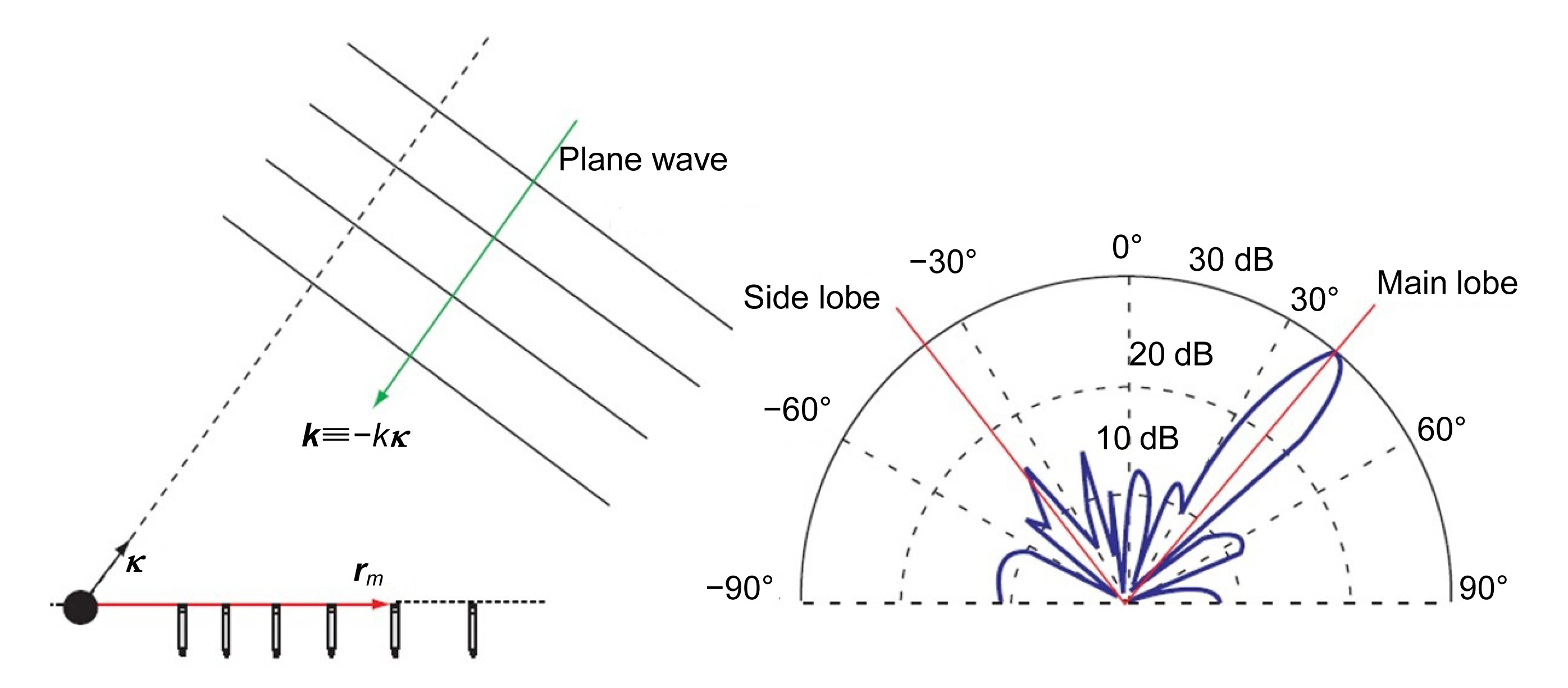
As illustrated in Fig. 1, when a planar array consisting of M microphones at locations rm is applied for both the localization and separation of the noise sources, the measured sensor signals ym are individually delayed and subsequently summed (Johnson and Dudgeon, 1993):
,
where κ is a unit vector, t is transient time, wm is the weighting or shading coefficient applied to the microphone signal, and Δm is the time delay, the value of which is obtained by adjusting the time delays such that the sound signals are associated with a plane wave incident from that specific direction. The signals are time-aligned before being summed. As shown in Fig. 1, geometrical considerations indicate that the time delays can be obtained by
,
where c is the speed of sound. The sound signals arriving from other far-field directions are not aligned before their summation, and are therefore not added up coherently. The frequency-domain version of Eq. (1) for the delay and sum beam-forming method is expressed as
,
where Ym(ω) is the frequency-domain sound pressure expression of the mth microphone, is the angular frequency, and k is the wavenumber vector of a plane wave incident from the focus direction κ.
Fig.1 Basic principle of external sound source localization (Christensen and Hald, 2004) k is the amplitude of k
The presence of side lobes can cause waves from unfocused directions to leak into the main lobe direction κ, resulting in false noise sources. A good planar array design can overcome this weakness. The performance of the beam-forming array is determined by the array pattern, the spatial resolution, and the maximum side lobe levels (MSLs). When a plane wave with a wave vector k0 arrives from a direction different from the focus direction, the pressure measured by the array sensors is given by
,
where Y0 is the pressure amplitude. According to Eq. (3), the output in the frequency domain is
.
Assuming that K=k−k0, the function W can be expressed by
.
This expression is the so-called array pattern and represents the amount of “leakage” obtained from plane waves incident from other directions, being something that strongly depends on the array geometry.
The ability of a beam-forming array to distinguish incident waves from various directions is indicated by its resolution. Under the assumption that two waves with wave vectors k1 and k2 have a unitary amplitude, the output can be expressed as
.
Then, considering a small angle difference dθ between k1 and k2, the resolution at a finite distance z is given by
,
where dK is the width of the main lobe in the array pattern, whose value is ,
θis the incident angle of the wave, and k is the amplitude of k1 and k2. It can be seen that the resolution deteriorates when the incidence angle increases. In practice, the useful open angle is typically restricted to 30°.
Another important parameter is the side lobe magnitude. For existing side lobes, waves from unfocused directions leak into the measurement direction (the main lobe direction), resulting in the possible production of false noise sources. A good planar array design can therefore be characterized by a low MSL. The radial profile of the array pattern is defined by
.
Furthermore, based on this expression, the MSL function can be written as
,
where is the width of the main lobe. For low MSL values, the array will exhibit a better performance. In this test, an optimized wheel microphone array with 78 channels is used (Fig. 2). Its geometrical design has improved the spatial resolution and reduced the MSL. The microphones are arranged in a series of tilted linear spokes. In practice, such a wheel array has an excellent performance and is easily operated.
Fig.2 Microphone array measurement setup
2.2. Measurement of high-speed train noise sources
The beam-forming method can effectively locate noise sources in the far-field (Kook et al., 2000). Hence, to measure the noise emitted from a train passing at high speed, the microphone array with 78 channels is placed at a horizontal distance of 7.5 m from the center line of the track (Fig. 2). The diameter of the array is 4.0 m and the height of the array center is located 2.0 m above the rail head. A photoelectric sensor is installed to measure the speed of the train. The speed is determined by calculating the ratio of the measured train length to its pass-by time. Processing of the measurement data is conducted using B&K devices.
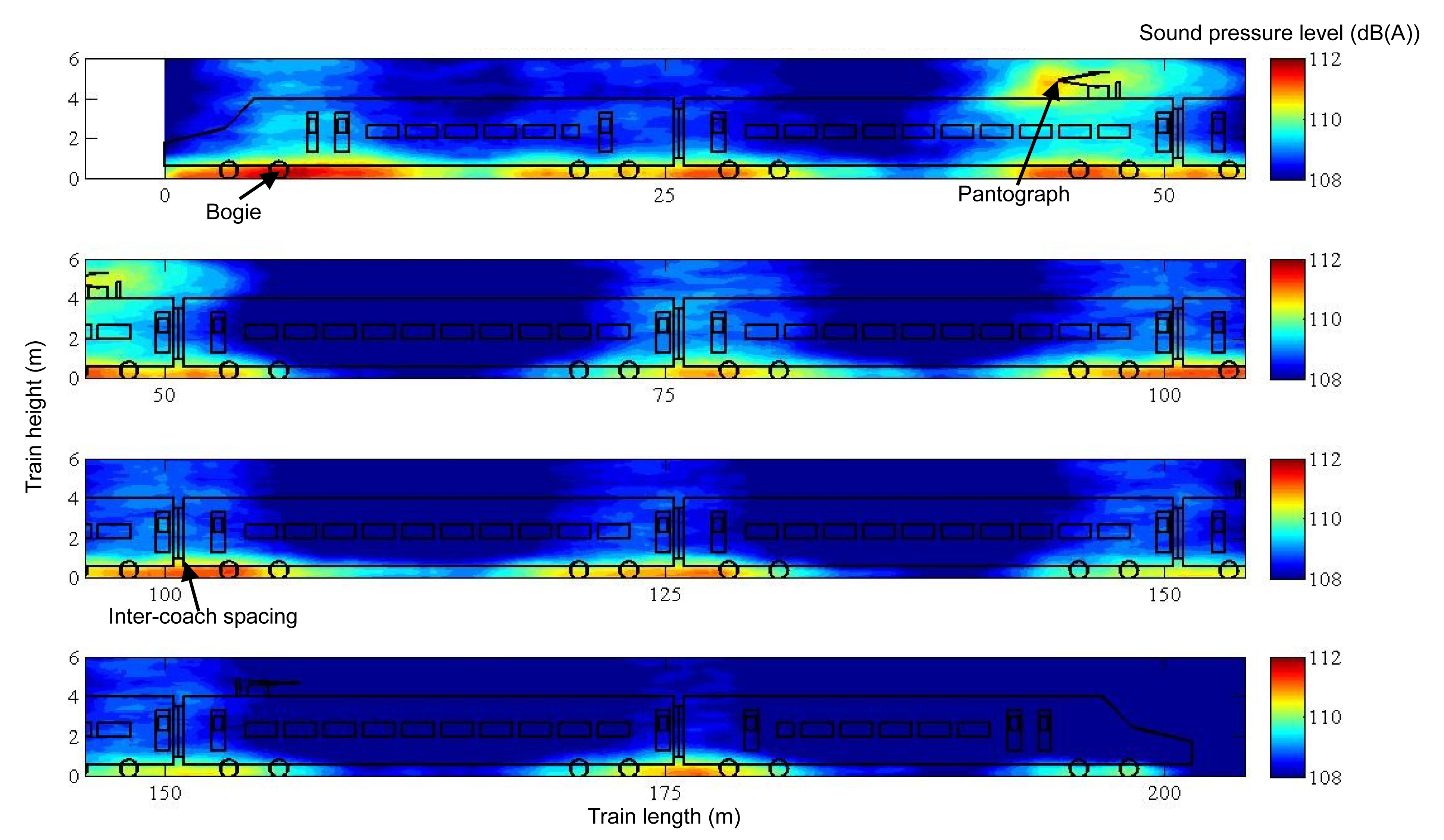
The test speeds range from 270 km/h to 390 km/h. Fig. 3 indicates the distribution of the external noise sources of the train at 386 km/h, which is identified by the microphone array discussed above. The frequency range of the noise shown in Fig. 3 is from 500 Hz to 5000 Hz, being the frequency range in which main external noise components are present. From the noise map, it can be deduced that the main noise sources over the entire frequency range are located at the bogies, the elevated pantograph, and the inter-coach gaps (Fig. 4).
Fig.3 Noise source distribution of a high-speed train traveling at 386 km/h on viaduct (frequency range: 500–5000 Hz)
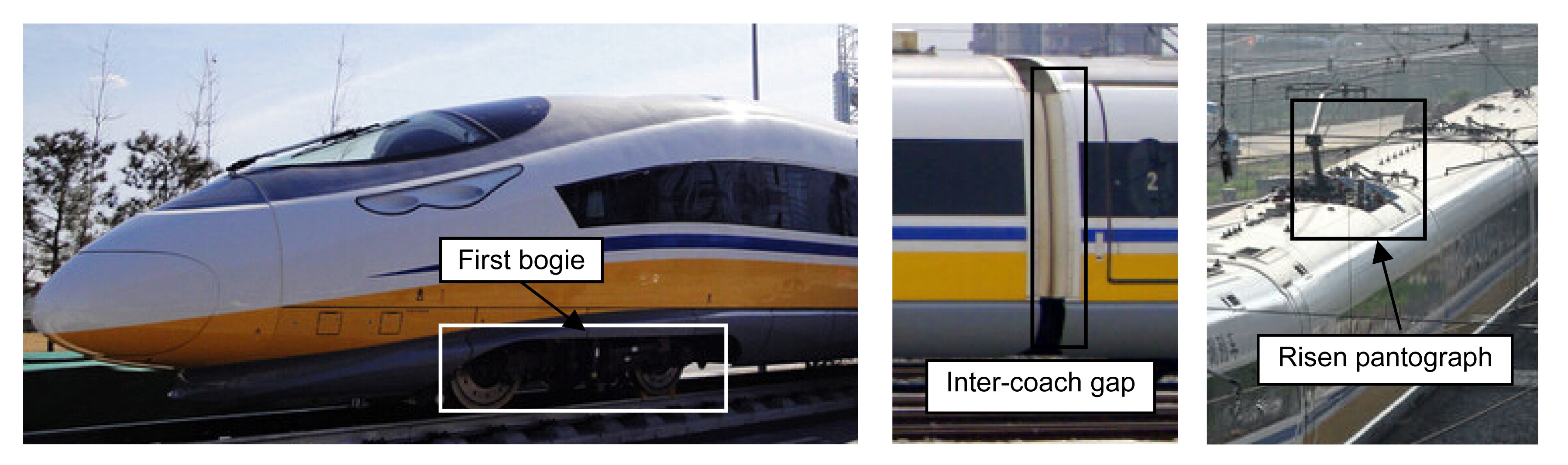
Fig.4 Noise sources: the first bogie, inter-coach gap, and pantograph
The maximum noise comes from the bogie areas, followed by the pantograph and inter-coach gap areas. The noise generated from the bogie areas includes the wheel/rail rolling noise, gear noise, and aerodynamic noise generated at the bogies under the carriages. The wheel/rail rolling noise is caused by the surface roughness of the wheels and the rails, and their mutual friction at the running surface. The gear noise is caused by the meshing impact and friction between the gears, and structural vibrations. The aerodynamic noise originates from the airflow around the entire bogie, including the influence of severe turbulence due to the complex geometry of the bogie. The noise coming from the bogie areas also includes contributions from structural vibrations. However, in these bogie areas, the wheel/rail rolling noise is always the dominant noise source when the train is moving although, so far, it has been very difficult to accurately identify to which extent (by percentage) each noise source contributes to the overall noise coming from the bogie area.
The noise in the pantograph area mainly includes aerodynamic noise, friction noise, and sparking noise. The aerodynamic noise is generated from interactions of the pantograph frame and shield with the airflow around them. The frictional noise is caused by the pantograph collector sliding on the catenary, while the sparking noise is produced by interaction between the collector and the catenary. In the pantograph area, the aerodynamic noise contribution is the greatest, followed by the sparking noise. As is the case for the bogie areas, it is also difficult to accurately identify the contribution percentages of each source in the overall noise generated in this area.
The noise of the inter-coach gaps includes aerodynamic noise and noise coming from structural vibrations. In this regard, the aerodynamic noise is the dominant source, due to the sags and crests of the outer windshield surfaces in the inter-coach gaps.
Hence, the external noise emitted by high-speed trains can be divided into two main source families: rolling noise and aerodynamic noise. The rolling noise is one of the most important noise sources of high-speed trains and is caused by the excitation at the wheel/rail contact patch. The aero-acoustic sources are generated by vortex shedding and flow disturbances around the train structure; these are mainly located at the bogies, the pantograph and its recess, the inter-coach gaps, and the doors.
Fig. 3 shows that the noise produced at the first bogie of the train is evidently greater than that at the other bogies. Obviously, when the train is running at high speed, the vortex shedding from the first bogie generates a much larger aerodynamic noise than the other bogies. From the color map shown in Fig. 3, it can be seen that the noise from the inter-coach gaps is mainly distributed underneath the coach roof and on the apron board. In these two areas, no windshields are used to decrease flow disturbances at the coach edges and the gaps (Fig. 4). Note that the color map in Fig. 3 is a summation of every 1/3 octave frequency-band results and represents the overall noise distribution. However, the predominant noise components of the noise sources vary for different frequency ranges and train speeds.
Other results involving external noise measurements are shown in Fig. 5, in which the noise distribution of the first two coaches is highlighted at 630, 1600, and 5000 Hz.
Fig.5 Noise distribution of the first two cars at 386 km/h with the frequency of 630 Hz (a), 1600 Hz (b), and 5000 Hz (c)
At 630 Hz, the noise sources are mainly located at the bogies and consist mainly of rolling and gear noises, which are produced by wheel/rail contact and friction/meshing mechanisms, respectively. At 1600 Hz, the noise is mainly located at the bogies and is formed by wheel/rail contact. Lastly, at 5000 Hz, noise is mainly located at the train body and inter-coach gaps, and is caused by flow disturbance around the train structure and vortex shedding. Hence, the dominant noise sources differ in all three analyzed frequencies. Similar results have been reported in previous studies (Koh et al., 2007; Thron, 2010; Noh et al., 2011). Distinction between the test results discussed in this study and those in previous studies are attributed to the train type and its operational speed. The train type affects the intensity, distribution, and frequency characteristics of the noise sources. Furthermore, as the train velocity increases, the aerodynamic noise becomes more significant, especially at high frequencies. Thus, for a speed of 386 km/h, the noise source intensity at 5000 Hz changes negligibly and does not depend on the height.
2.3. Frequency characteristics of main noise sources
The previous section provided a qualitative analysis of the noise sources, their locations, and their relative intensity. In this section, a quantitative analysis of the frequency characteristics of the main noise sources is provided, in which the noises at the bogies, the elevated pantograph, and the inter-coach gaps are being considered. The formula for averaging the noise pressure can be expressed as
,
where s is the area of the analyzed region, p is the A-weighted sound pressure in the considered area, p0 is the reference sound pressure, Ni and Nj represent discrete points, and dy and dz represent the increment of diversity along the length and the height directions, respectively. The analyzed regions and their areas for the three noise sources have been documented elsewhere (He, 2010). When combined with the source regions, the intensity of the three noise sources can be evaluated. As the sound pressure at a given field point is an average value, the average sound pressure Lp deserves more attention, since this data is also used as the sound source in noise prediction models.
The frequency characteristics of the three sources are shown in Figs. 6–8, corresponding to speeds given by 271, 341, and 386 km/h, respectively. When the speed is 271 km/h, the average sound pressures in the wheel/rail areas, the pantograph area, and at the inter-coach gaps are 106.2, 104.2, and 104.3 dB(A), respectively. The sound pressure increases as the frequencies increase, peaking at 1600 Hz with values of 99.5, 95.9, and 95.0 dB(A) for the wheel/rail areas, the inter-coach gaps, and the pantograph area, respectively. Below 1600 Hz, the noise originating at the wheel/rail area is the largest, followed by the inter-coach gap noise and the pantograph noise. The maximum pressure difference between the noises originating at the wheel/rail area and the inter-coach gaps is approximately 6.8 dB(A). The pressures at frequencies above 3150 Hz are very similar, with a maximum value of approximately 97.7 dB(A).
Fig.6 Frequency characteristics of the main noises at 271 km/h (frequency range: 500–5000 Hz)
Fig.7 Frequency characteristics of the main noises at 341 km/h (frequency range: 500–5000 Hz)
Fig.8 Frequency characteristics of the main noises at 386 km/h (frequency range: 500–5000 Hz)
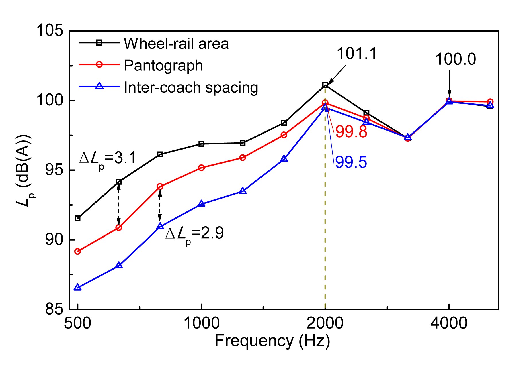
For a speed of 341 km/h, the average sound pressures in the wheel/rail areas, the pantograph area, and the inter-coach gap areas are 108.5, 107.7, and 107.0 dB(A), respectively. The sound pressures reach their maxima at 2000 Hz, with values of 101.1, 99.8, and 99.5 dB(A) for the wheel/rail areas, the pantograph area, and the inter-coach gap areas, respectively. Below 2000 Hz, the noise coming from the wheel/rail areas is the highest, followed by the noise originating at the pantograph area. The noise at the inter-coach gaps has the smallest contribution in this frequency range. The maximum pressure differences between them are approximately 3.1 and 2.9 dB(A). The resulting pressures above 3150 Hz are quite similar, with a maximum value of 100.0 dB(A).
Finally, for a train velocity of 386 km/h, the average sound pressures in the wheel/rail areas, the pantograph area, and the inter-coach gap areas are 110.4, 110.3, and 109.0 dB(A), respectively. The largest sound pressure, at approximately 102.4 dB(A), is reached at 5000 Hz. At 2500 Hz, there are local sound pressure peaks with values of 100.7, 100.4, and 99.8 dB(A) for the wheel/rail areas, the pantograph area, and the inter-coach gap area, respectively. Below 2500 Hz, the wheel/rail area is the largest noise contributor, followed by the pantograph areas and the inter-coach gap area. Above 3150 Hz, the measured pressures are very similar, with a maximum measured value of approximately 102.4 dB(A).
From the above analysis, it can be seen that for low train velocities, the average noise pressure coming from the wheel/rail areas is the largest, while the noise pressure produced by the inter-coach gaps takes the second place. As the speed increases, the average pantograph noise exceeds that of the inter-coach gaps. When the speed is 386 km/h, the noise produced in the wheel/rail areas is still the largest, although the noise produced in the pantograph area is almost consistent with that from the wheel/rail areas. Furthermore, as the velocity increases, the frequency of the maximum noise moves to higher values. In this regard, for speeds of 271, 341, and 386 km/h, the maximum noise is measured at 1600, 2000, and 5000 Hz, respectively.
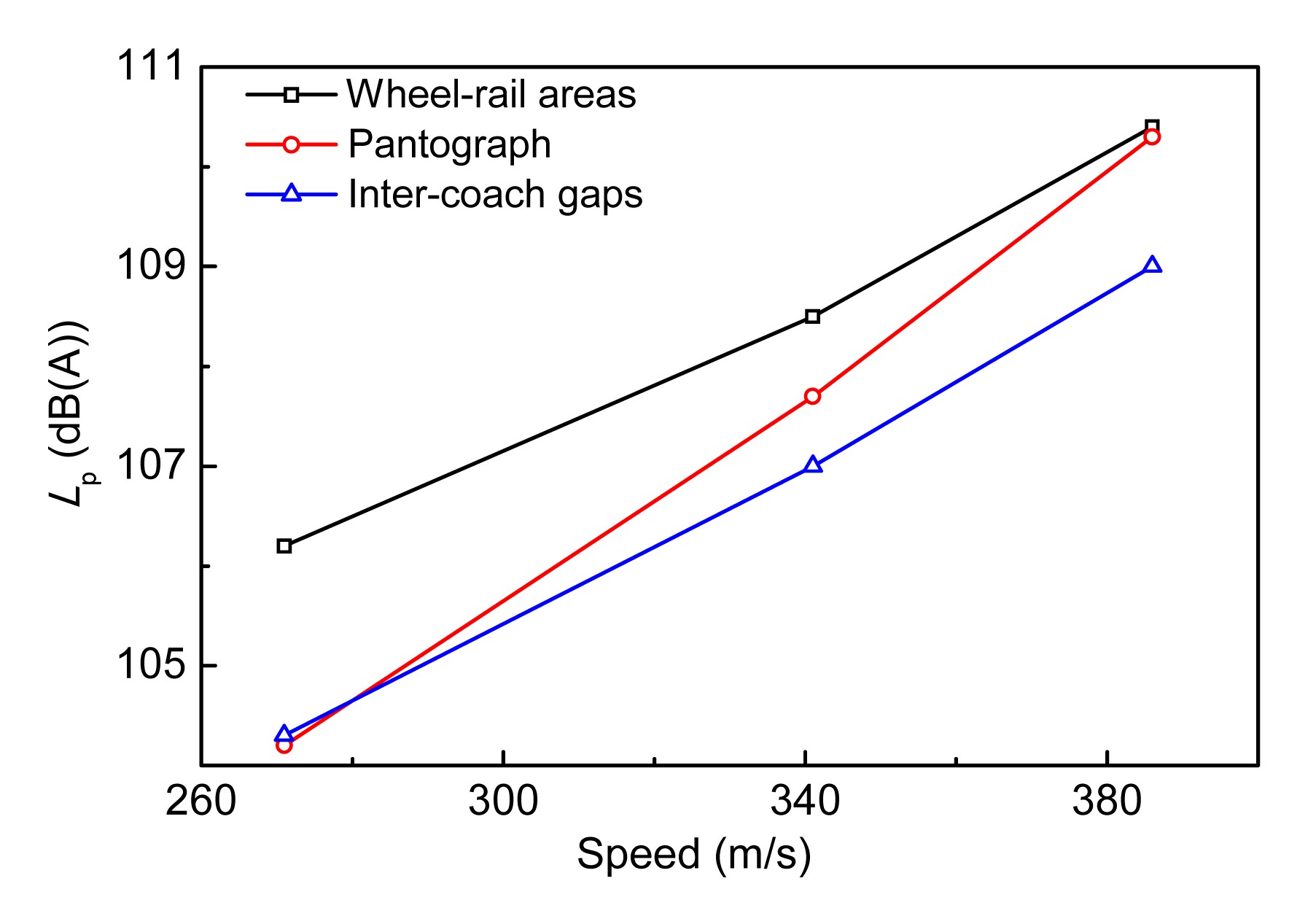
Fig. 9 shows the average pressures of the three noise sources as a function of the train speed. The aerodynamic noise at the pantograph area increases faster than the other two noise sources. So the power law relationship for this area between noise and train speed is larger than that for other areas. The wheel/rail noise contains rolling noise and aerodynamic noise, so the produced average sound pressure in this area is higher than that of the inter-coach gap areas. From the sound levels and the spectrum of the three noise sources, it can be seen that for a speed of 271 km/h, the major noise type generated in the wheel/rail areas is rolling noise. However, as the train speed increases, the share of the aerodynamic noise in the wheel/rail noise is greater. For a velocity of 386 km/h, the aerodynamic noise in wheel/rail areas approaches the rolling noise.
Fig.9 Sound pressures vs. speed
2.4. Characteristics of SEL at different speeds
The vertical noise distribution of high-speed trains reflects the intensity of noise sources in the vertical direction along the train and is expressed by the SEL. This quantity measures the energy contained in transient noise. According to the ISO 3095:2013 standard (ISO, 2013), the formula to calculate the SEL is given by
,
where T0 is the reference time interval (T0=1 s), pA(t) is the A-weighted instantaneous sound pressure, p0 is the reference sound pressure, and T is the measurement time interval.
Figs. 10–12 show the SEL distribution along the vertical height direction for train velocities of 271, 341, and 386 km/h, respectively. The parameter T is the pass-by time of the high-speed train. The abscissa represents the value of the SEL, the ordinate represents the vertical height, and the height coordinate corresponding to 0 indicates the height of the rail head.
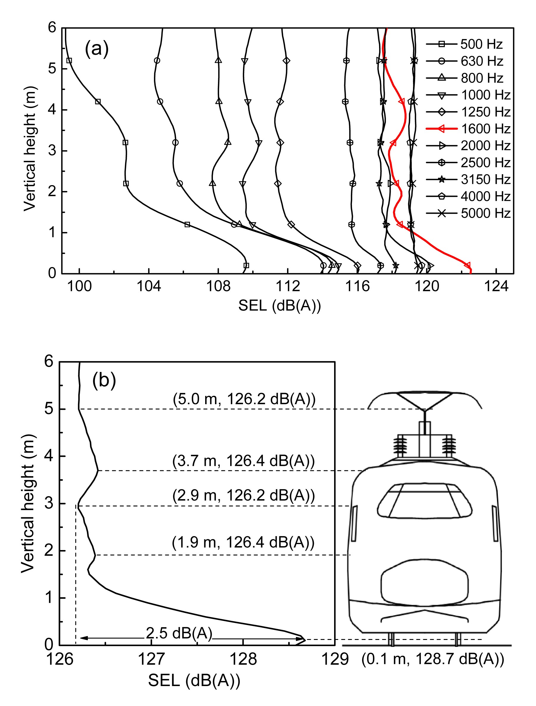
Fig.10 SEL distribution at 271 km/h (a) SEL in every 1/3 octave frequency band; (b) SEL in the full frequency range
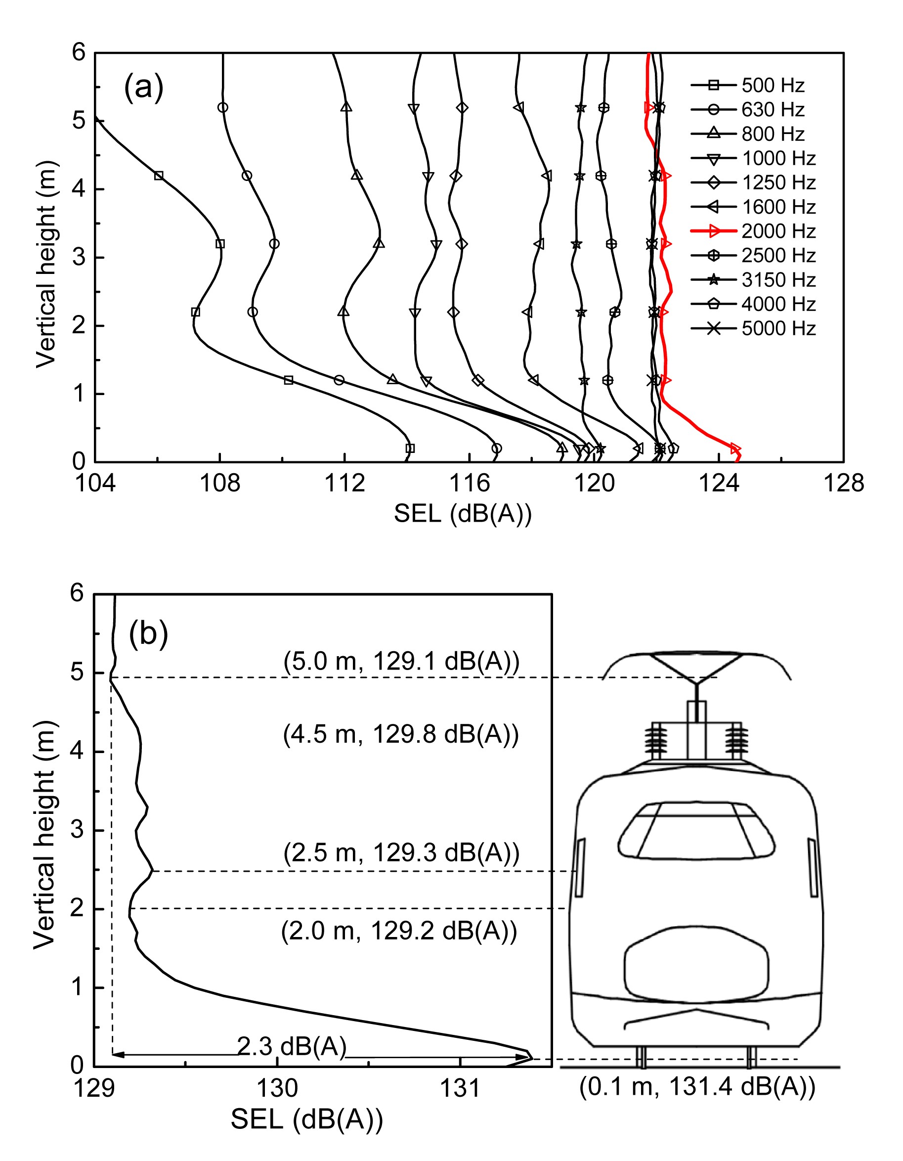
Fig.11 SEL distribution at 341 km/h (a) SEL in every 1/3 octave frequency band; (b) SEL in the full frequency range
Fig.12 SEL distribution at 386 km/h (a) SEL in every 1/3 octave frequency band; (b) SEL in the full frequency range
The vertical distribution of the SEL in the frequency range of 500–5000 Hz is illustrated in Fig. 10a for a train speed of 271 km/h. It can be clearly observed that in every 1/3 octave frequency band, the SEL corresponding to the wheel/rail area within a height of 1.0 m is the highest. Below 1600 Hz, SEL values of all heights increase as the frequencies increase. Furthermore, the SELs at 4000 and 5000 Hz are approximately similar, showing negligible variation along the vertical direction. At a height of 1.0 m, the SEL at 1600 Hz is maximized, and can be attributed to wheel/rail noise. Above 1.0 m, the SELs corresponding to 4000 and 5000 Hz exhibit the largest values. As revealed by the noise source identification, it is known that the main noise contributor corresponding to these frequencies is aerodynamic noise produced by the pantograph, the bogies, the inter-coach gaps, and the first access door. Fig. 10b shows the total SEL values for a speed of 271 km/h. Here the maximum SEL is 128.7 dB(A), corresponding to a height of 0.1 m. At the base of the pantograph, a local maximum SEL is observed with a value of 126.4 dB(A). The minimum SEL value is 126.2 dB(A) and is measured at heights given by 2.9 and 5.0 m, corresponding to the center of the train body and the pantograph, respectively. Hence, during the pass-by time, the total SEL is maximized in the wheel/rail region, followed by the inter-coach gaps and the pantograph. Furthermore, the SEL difference between the wheel/rail area and the pantograph (from the bottom up) is 2.5 dB(A), being the maximum measured SEL difference.
As shown in Fig. 11a, for a speed of 341 km/h, SEL values below 1.0 m exhibit the largest values for every 1/3 octave frequency band. This is attributed to the contribution of intensive wheel/rail noise. Below 2000 Hz, the SEL increases along all heights as the frequencies increase. The SEL at 4000 and 5000 Hz are approximately equal and only change little along the vertical direction. Below 4.5 m, the SEL at 2000 Hz is larger than the values corresponding to 4000 and 5000 Hz. This is due to a large noise contribution at this frequency from the wheel/rail area and the carriage structure. Above 4.5 m, the contrary is the case, something that can be attributed to the large aerodynamic noise generated by the pantograph at 4000 and 5000 Hz. Fig. 11b shows the total SEL for a speed of 341 km/h, showing a maximum SEL of 131.4 dB(A) located 0.1 m above the rail head. Two local SEL minima are found at a height of 2.0 m and at the pantograph with values given by 129.2 and 129.1 dB(A), respectively. Hence, the largest SEL is obtained in the wheel/rail area, while the SELs corresponding to the regions of the pantograph and the inter-coach gaps are similar to each other. For a speed of 341 km/h, the maximum SEL difference is obtained between the wheel/rail area and the pantograph (from the bottom up) and equals 2.3 dB(A).
Similarly to Figs. 10a and 11a, Fig. 12a shows that the SELs corresponding to a train velocity of 386 km/h are maximized below a height of 1.0 m for every 1/3 octave frequency band. However, in this case the SELs at all heights increase for larger 1/3 octave frequency bands. The SEL at 5000 Hz is the highest compared to all other frequencies. From the results obtained for the source identification, it became apparent that the main noises at this frequency are of an aerodynamic nature, originating at the pantograph, the inter-coach gaps, and the first access door.
Fig. 12b shows the total SEL for a train moving at 386 km/h, with a maximum SEL value of 133.1 dB(A) that again occurs at a height of 0.1 m relative to the rail head. The minimum SEL is 131.0 dB(A) and is obtained at the pantograph. The total SEL difference above 1.0 m lies within 0.1 dB. Hence, the total SEL at the wheel/rail is the largest, while the SEL values measured at the pantograph and the inter-coach gaps are very similar. Lastly, the maximum SEL difference is 2.1 dB(A) and is between the wheel/rail area and the pantograph.
The SEL discussed above reflects the characteristics of the sound energy distribution along the vertical height of the high-speed train during the pass-by time. For low frequencies, the observed SEL difference is larger in this direction, since the noise mainly comes from the wheel/rail regions. As the frequency increases, the aerodynamic noise in the high frequency range that is caused by the train body, the inter-coach gaps, and the pantograph starts to emerge. Table 1 depicts the maximum SEL differences for each 1/3 octave frequency band. From the results shown in Figs. 10–12 and Table 1, it can be deduced that the frequency corresponding to the maximum sound energy increases with increasing train velocity. In every 1/3 octave frequency band, the SEL exhibits its maximum in the wheel/rail region, especially at a height of 0.1 m above the rail head. As the frequency and the speed increase, the aerodynamic noise caused by disturbed flow and turbulence emerges along the entire height, resulting in a decrease of the maximum SEL differences by 9.3–9.9 dB among the analyzed frequency components that range from 500 Hz to 5000 Hz. For the full frequency range, the maximum SEL differences in the vertical direction equal 2.5, 2.3, and 2.1 dB for speeds of 271, 341, and 386 km/h, respectively. Hence, the SEL difference along the vertical direction decreases as the train speed increases. A similar result has been reported in another study (Bernd et al., 2002). Furthermore, faster train speeds also push down the ratio between the wheel/rail noise and the aerodynamic noise.
Table 1
Maximum SEL differences at different train speeds and different frequencies
Frequency (Hz)
Maximum SEL difference (dB(A))
v=271 km/h*
v=341 km/h
v=386 km/h
500
10.4
10.6
9.6
630
9.7
8.8
8.5
800
6.9
7.4
6.8
1000
5.5
5.4
5.4
1250
4.8
4.5
4.6
1600
5.1
4.0
4.0
2000
3.0
3.0
2.6
2500
2.1
2.0
1.9
3150
1.0
0.9
0.9
4000
0.8
0.7
0.6
5000
0.5
0.4
0.3
Overall SEL
2.5
2.3
2.1
*
v is the operating speed of the train
3. Pass-by noise magnitude and its characteristics
When noises generated by different sources of a high-speed train radiate outward based on their precise characteristics (especially directivity) and reach different field points, the corresponding sound pressure responses can be measured. The sound pressure levels at standard measuring points are important for evaluating the noise of high-speed trains. In the ISO 3095:2013 standard, M1 (7.5 m, 1.2 m), M2 (7.5 m, 3.5 m), and M3 (25 m, 3.5 m) are three specified field points. The numbers in brackets represent the distances with respect to the center line of the track and the height of the rail head.
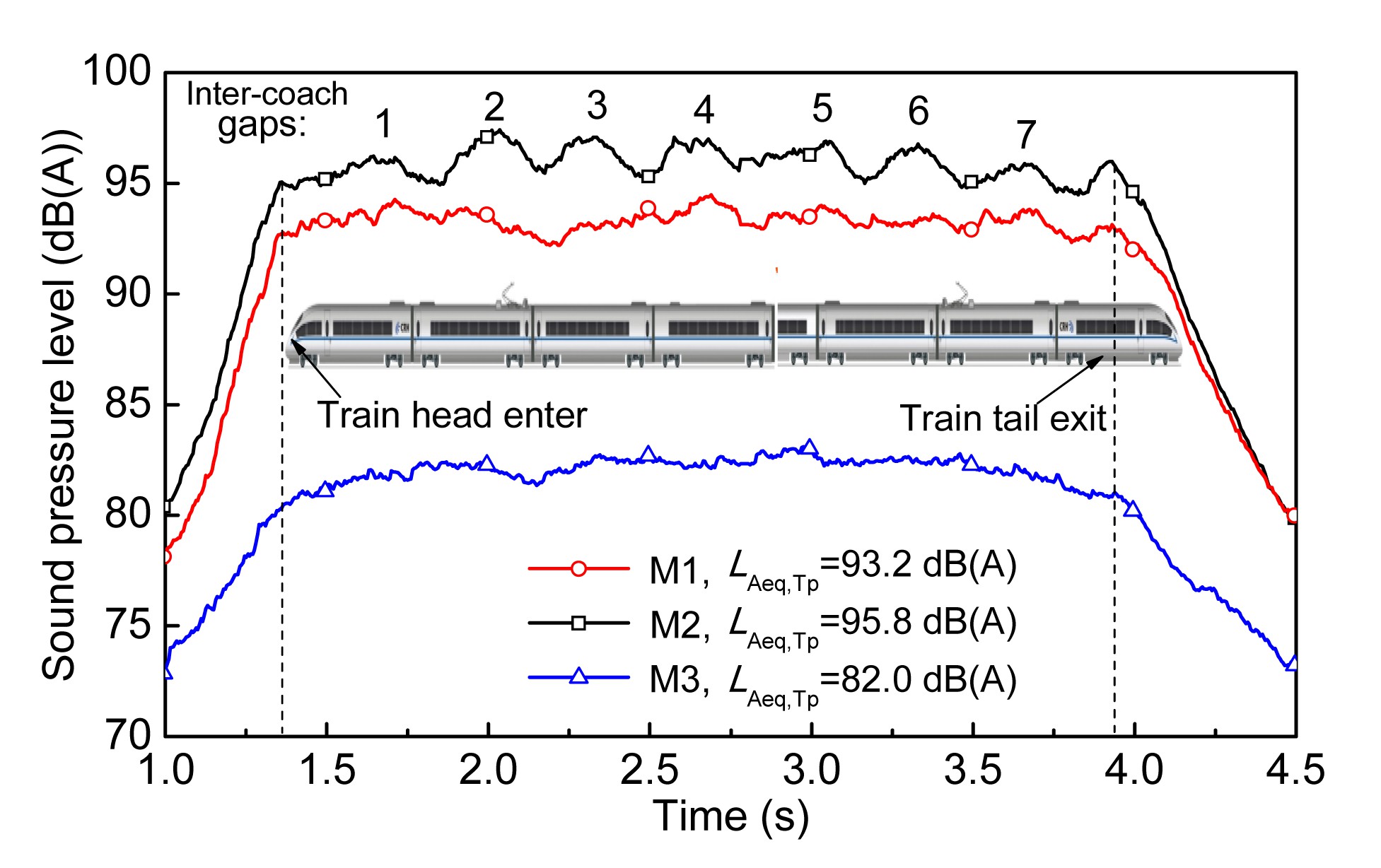
Fig. 13 illustrates the time histories of the sound pressure levels of the high-speed train measured at M1, M2, and M3, obtained during a single pass-by at 271 km/h. These results can be used for further identification of the noise sources. The time histories of field points M1 and M2 have a strong correlation with the characteristics of the train structure, showing nine sound pressure peaks (Fig. 13). The first peak corresponds to the entrance of the train head, while the last peak is attributed to the exit of the train tail. The seven peaks between them represent the seven gaps between the eight coaches, making the number of observed valleys equal to the number of coaches. It is confirmed that the pressure peaks are predominantly generated at the train head, the train tail, the bogie areas, and the inter-coach gaps. Note that the pantograph is located close to one of the inter-coach gaps (Fig. 13). During the pass-by time, the highest noise pressure level is measured at M2, subsequently followed by M1 and M3. This situation is closely related to the characteristics of the near field sound directivity, except for the aerodynamic noise generated in the inter-coach gaps, the pantograph, and the bogies.
Fig.13 Time histories of the sound pressure levels during a single pass-by of a high-speed train at 271 km/h
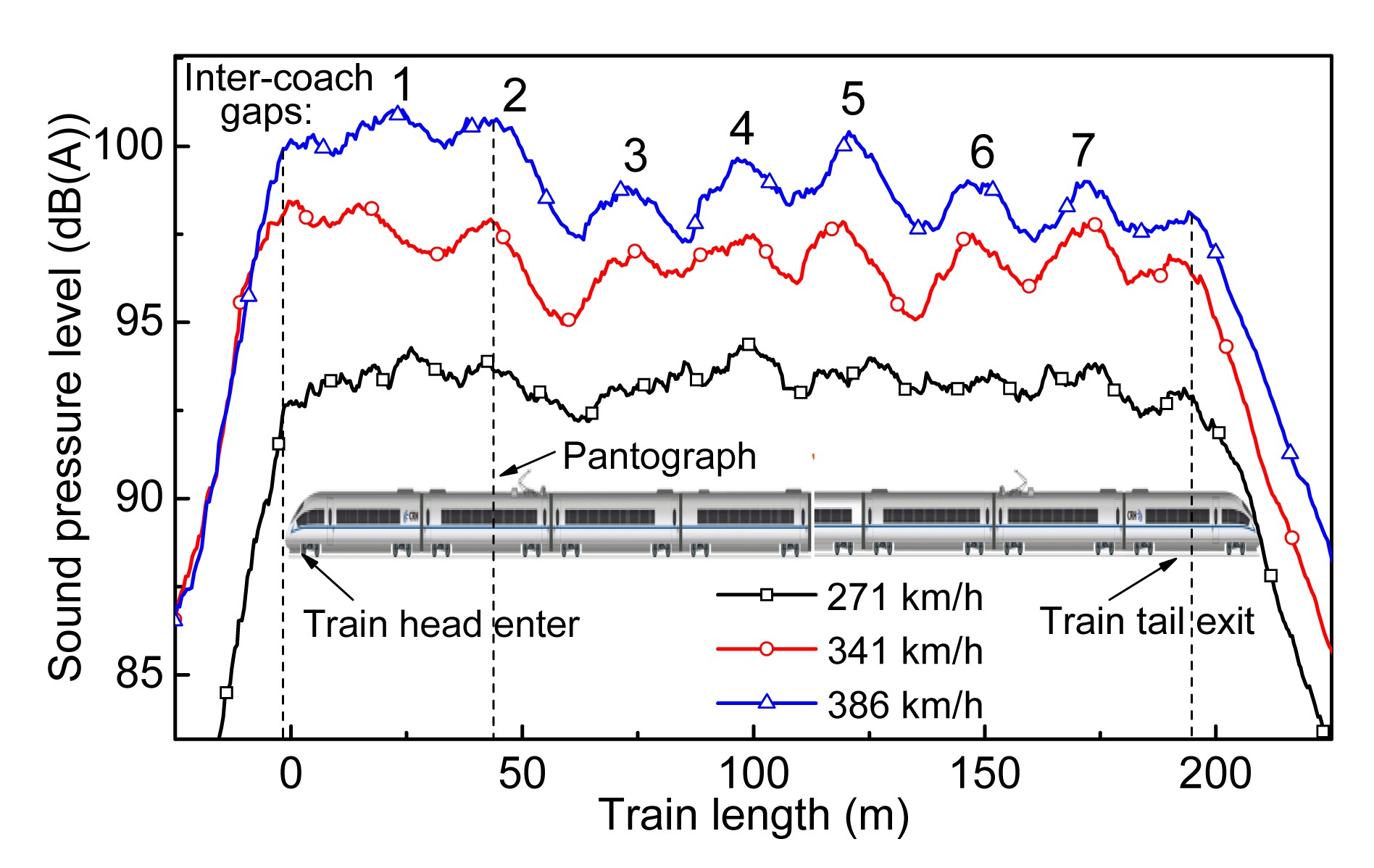
Fig. 14 depicts the time histories of the sound pressure levels measured at M2 for different speeds. The noise peak distribution and its qualitative explanation are similar to the results shown in Fig. 13. The noise peak caused by the pantograph is the third peak located near the second inter-coach gap. For a train speed of 271 km/h the maximum noise during a single pass-by is caused by the fourth inter-coach gap, close to the wheel/rail region. When the speed is 341 km/h, the maximum noise comes from the train head and the first bogie region. The noise peak caused by the second inter-coach gap and the pantograph is larger than all other peaks, except for the first and second peaks. When the speed is 386 km/h, the second and third peaks are dominant, corresponding to the first inter-coach gap, and the combination of the second inter-coach gap and the pantograph, respectively.
Fig.14 Time histories of the sound pressure level at M2 at different speeds
As the speed increases, it can be seen that the noise caused by the first two coaches increases, becoming significantly larger than the noises caused by all other coaches. The main reason for this is the fierce interaction of airflows with the first bogie, the pantograph, and the first two inter-coach gaps, thus generating a strong aerodynamic noise around these structures when the train travels at higher speeds.
The A-weighted equivalent continuous sound pressure level (LAeq,Tp) reflects the average noise energy during the pass-by time. Table 2 shows these values at the three field points M1, M2, and M3 for different train speeds, while Fig. 15 depicts the frequency characteristics of the noise pressures at these three field points for different speeds. The frequency range shown in Fig. 15 goes from 160 Hz to 10 000 Hz, covering the main external noise frequencies of the train. The sound sources spread through the air, and subsequently cause a response at the field points. According to sound propagation theory, the sound pressures measured at the field points are closely related to the frequency, the directivity of the sound source, and the environment of the sound field (airflow, temperature, humidity, terrain, etc.). Thus, the frequency characteristics of the field points are not solely determined by the frequency characteristics of the sound sources. The pressure levels detected at the field points increase with increasing speeds. For equal velocities, the noise level at M3 is approximately 10.0–13.0 dB lower than that at M1 and M2.
Table 2
Sound pressure levels of M1, M2, and M3 at different speeds
Speed (km/h)
LAeq,Tp (dB(A))
M1
M2
M3
271
93.2
95.8
82.0
341
96.5
98.0
85.5
386
98.5
100.1
88.1
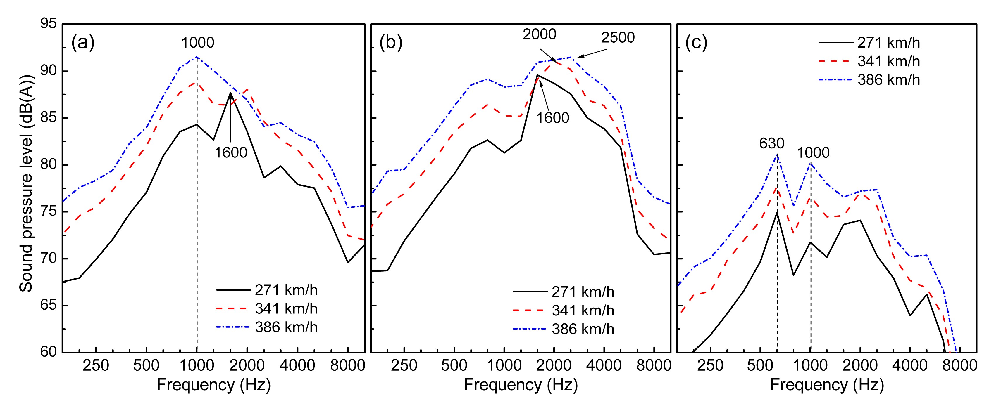
Fig.15 Frequency characteristic of three field points at different speeds: (a) M1; (b) M2; (c) M3
As shown in Fig. 15a, at M1, for a speed of 271 km/h the noise is maximized at 1600 Hz, while for velocities of 341 and 386 km/h this happens at 1000 Hz. However, when analyzed as a function of the speed, the noise level at 1600 Hz does not change significantly and the peak disappears for larger velocities. For M2 (Fig. 15b), the noise component characteristics at 1600 Hz are similar to those measured at M1, while the noise levels corresponding to speeds of 341 and 386 km/h reach their maxima at 2000 and 2500 Hz, respectively. At both M1 and M2, the noise components measured at 1600 and 2000 Hz do not change much as a function of the train velocity. At M3 (Fig. 15c), the levels of all noise components increase with increasing speeds along the entire analyzed frequency range.
Since the measuring points M1 and M2 have the same distances with respect to the center line of the track, but different distances with respect to the rail head, their frequency characteristics are different, which is exemplified in Figs. 15a and 15b. The main difference is that the dominant components of the noise or the peak frequencies move forward. At M1 the noise components from 600 Hz to 2000 Hz are predominant, while at M2 the dominant noise components are distributed between 1600 and 4000 Hz. This is caused by the fact that M1 is located close to the wheel/rail area, hence demonstrating that noise generated in this area has a greater contribution to the measured results, when compared to other noise sources. However, M2 is located near the pantograph, the carriage body, and the inter-coach gaps. Since at these regions much aerodynamic noise is generated, this demonstrates that this noise type greatly contributes to the measured results at M2, when compared to other noise sources.
When comparing the results at M1, M2, and M3, it can be concluded that the results measured at M1 and M2 are quite similar. Although the heights of M2 and M3 are approximately the same, at M3, which is placed at a much larger distance from the central line of the track, the wheel/rail noise has a much larger contribution to the total noise level, when compared to the aerodynamic noise. At this measurement point, the dominant noise components range from 600 Hz to 2500 Hz and their characteristics clearly change with increasing train speeds. Usually, these noise components mainly consist of wheel/rail noise. Hence, for moving high-speed trains, the control and reduction of wheel/rail rolling noise should be considered first.
Fig. 15 clearly shows that the differences in level of the noise components at points M1, M2, and M3 have the tendency to decrease for larger frequencies and increasing speeds. This explains that the aerodynamic noise of the train increases in an extensive frequency range as the train velocity becomes larger. In addition, Fig. 15 shows that the noise components at 630, 1000, 1600, 2000, and 2500 Hz are always activated. Their precise generation mechanisms, which up to this point are not known, will be further investigated.
To effectively reduce the external noise, the maximum noise in the full frequency range, the location of its source, and the mechanism generating it should first be clearly identified. Taking M3 as an example, maximum noise peaks occur at 630 and 1000 Hz. From Fig. 12, it can be deduced that the SEL below a vertical height of 1.0 m is about 9.0 and 5.0 dB larger than those at other heights for 630 and 1000 Hz, respectively. The vertical height of 1.0 m belongs to the wheel/rail area. Therefore, the noise generated in this area needs to be controlled and reduced preferentially. Major measures to suppress wheel/rail noise include the employment of a bogie skirt to reduce the aerodynamic noise, the use of damping measures for both wheels and rails to reduce rolling noise, and the installation of sound barriers to change the noise propagation path.
4. External noise behaviors as a function of speed
The characteristics of the noise radiated by high-speed trains can be established with an approximate function that depends on the train speed. The function can be approximated by a second-order polynomial of the variable lg(v) (Mellet et al., 2006). The regression equation can be expressed as
,
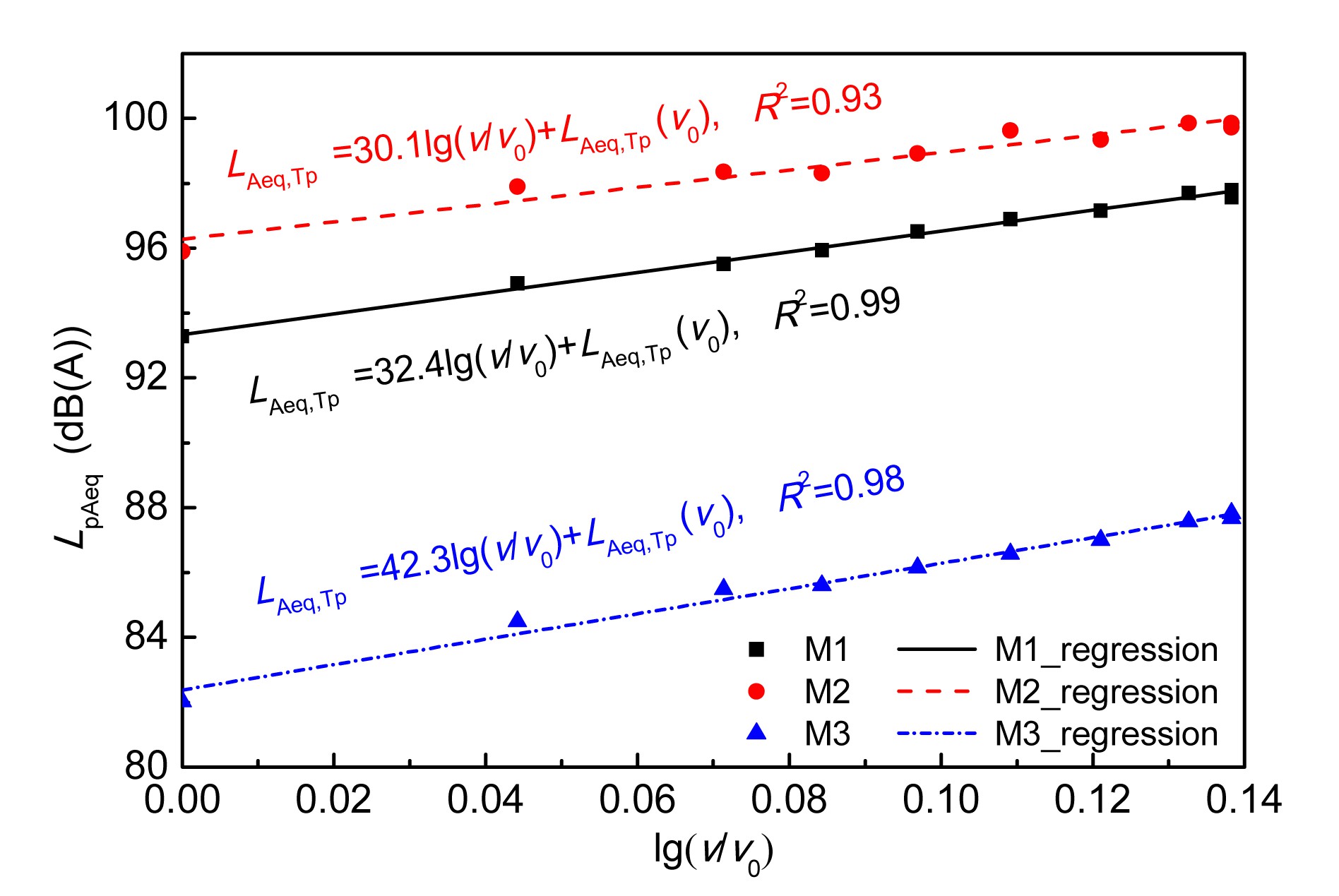
where A, B, and C are regression coefficients. For simplicity, this piecewise linear function can be used to replace the nonlinear function displayed in Eq. (13). According to the characteristics of the wheel/rail noise and the aerodynamic noise with respect to the train speed, the piecewise linear regression function is considered in two speed ranges, one being defined below 300 km/h, and the other above 300 km/m. The speed of 300 km/h is considered the break speed (Mauclaire, 1990; Krylov, 2001). Below 300 km/h, the slope of the linear function is approximately 30, while above the break speed a slope of 60 is found. For both speed ranges, 30 and 60 denote the regression coefficient B in Eq. (13). If the value of LAeq,Tp at the reference speed v0 is known, the linear regression law can be expressed as
.
Fig. 16 shows the linear regressions of LAeq,Tp for the three different field points. Note that from 280 km/h to 390 km/h, the regression coefficients B are 32.4, 30.1, and 42.3, while the corresponding correlation coefficients R2 are 0.99, 0.93, and 0.98 for M1, M2, and M3, respectively.
Fig.16 Linear regressions of the measured data from 280 km/h to 390 km/h (v0=280 km/h)
Using these measured results, it can be assumed that this linear expression is valid up to velocities of 390 km/h. The transition speed for which aerodynamic noise becomes as important as the rolling noise, which generally is considered to lie around 300 km/h (Mauclaire, 1990; Krylov, 2001), is not clearly observed. The regression coefficients for M1 and M2 are close to 30, a value which is commonly used in the prediction formula for wheel/rail rolling noise. Hence, the rolling noise is dominant when considering the total noise measured at M1 and M2 for a speed close to 390 km/h. For M3, the regression coefficient is approximately 42. To reduce the pass-by noise at this field point, one needs to take measures to suppress both rolling noise and aerodynamic noise, although the rolling noise still makes a greater contribution to the total noise detected at M3 compared with the aerodynamic noise.
5. Conclusions
This paper presents the test results and an analysis of external noise characteristics produced by a Chinese high-speed train traveling at different speeds. From this study, the following conclusions can be drawn:
External noise identification of the high-speed train shows that main noise originates at three areas: the wheel/rail systems (or bogies), the pantograph, and the inter-coach gaps. The wheel/rail area produces the dominant rolling noise and the aerodynamic noise caused by airflow around the bogie. The pantograph and the inter-coach gaps of the train mainly generate aerodynamic noise. For speeds below 386 km/h, the SEL of the wheel/rail area is the greatest in the frequency range below 3150 Hz, while the SELs of the three noise sources are quite similar for larger frequencies.
For both the total external noise and the predominant noise components analyzed at different frequencies, the wheel/rail noise has the greatest contribution compared with the aerodynamic noise sources located at the pantograph and the inter-coach gaps. The measured noise from the wheel/rail area mainly includes the wheel/rail rolling noise and the aerodynamic noise coming from the bogie area. However, it has so far been difficult to experimentally determine their exact relative proportions in the total noise.
Along the vertical train height, maximum noise levels are found in the wheel/rail area. At distances far from the central track line, the wheel/rail rolling noise still makes a greater contribution than the aerodynamic noise for the entire train velocity range analyzed.
The measured results at all field points show that the noise components from 630 Hz to 2500 Hz, which are typically attributed to wheel/rail rolling noise, always dominate. Therefore, it is suggested that the design of low-noise high-speed trains and external noise control should be focused on the control and reduction of this type of noise.
The measured results at all different field points clearly indicate that the noise level differences have a tendency to decrease with increasing frequencies and train speeds. This explains the growth of aerodynamic noise over an extensive frequency range as the train runs faster. In addition, the test results show that noise components at 630, 1000, 1600, 2000, and 2500 Hz are always activated. Nevertheless, their exact generation mechanisms are currently unknown and will be further investigated.
[1] Bernd, B., Daniel, R.D., Hanson, C.E., 2002. Noise Characteristics of the Transrapid TR08 Maglev System. Dot-vntsc-fra-02-13, US Department of Transportation, :
[3] Dittrich, M.G., Janssens, M.H.A., 2000. Improved measurement methods for railway rolling noise. Journal of Sound and Vibration, 231(3):595-609.
[4] He, B., 2010. Primary Investigation into External Noise Distribution Characteristics of High-speed Train and Damping Control Measures of Wheel. MS Thesis, (in Chinese), Southwest Jiaotong Univesity,Chengdu, China :
[5] ISO (International Organization for Standardization), 2013. Acoustics-railway Applications—Measurement of Noise Emitted by Railbound Vehicles, ISO 3095:2013. . ISO,Switzerland :
[6] Johnson, D.H., Dudgeon, D.E., 1993. Array Signal Processing: Concepts and Techniques. Prentice Hall,New Jersey :94-99.
[7] Koh, H., You, W., Kwon, H., 2007. Noise source identification of Korean high speed train. , The 14th International Congress on Sound and Vibration, Cairns, 1498-1503. :1498-1503.
[8] Kook, H., Moebs, G.B., Davies, P., 2000. An efficient procedure for visualizing the sound field radiated by vehicle during standardized pass by tests. Journal of Sound and Vibration, 233(1):137-156.
[9] Krylov, V., 2001. Noise and Vibration from High-speed Trains. Thomas Telford,London :78-85.
[10] Mauclaire, B., 1990. Noise Generated by High Speed Trains. , Proceedings of Internoise, Gothenburg, Sweden, 371-374. :371-374.
[11] Mellet, C., Ltourneaux, F., Poisson, F., 2006. High speed train noise emission: latest investigation of the aerodynamic/rolling noise contribution. Journal of Sound and Vibration, 293(3-5):535-546.
[12] Noh, H.M., Choi, S., Hong, S.Y., 2011. Designing a microphone array system for noise measurements on high-speed trains. Journal of the Korean Society for Railway, (in Korean),14(6):477-483.
[13] Poisson, F., Gautier, P.E., Letourneaux, F., 2008. Noise Sources for High Speed Trains: a Review of Results in the TGV Case. Noise and Vibration Mitigation for Rail Transportation Systems, Springer Berlin Heidelberg,:71-77.
[14] Schulte-Werning, B., Jger, K., Strube, R., 2003. Recent developments in noise research at Deutsche Bahn (noise assessment, noise source localization and specially monitored track). Journal of Sound and Vibration, 267(3):689-699.
[15] Silence, ., 2005. Report on Source Ranking on State of the Art Validation Platforms and Final Priorities for Research Effort. European Commission,Austria :
[16] Thompson, D., 2008. Railway Noise and Vibration: Mechanisms, Modelling and Means of Control. Elsevier,New York :3-9.
[17] Thron, T., 2010. A Contribution to the Noise Prediction Based on Recognized Metrological Model Parameters. PhD Thesis, (in German), Technical University of Berlin,Berlin, Germany :
[18] Wakabayashi, Y., Kurita, T., Yamada, H., 2008. Noise Measurement Results of Shinkansen High-speed Test Train (FASTECH360S, Z). Noise and Vibration Mitigation for Rail Transportation Systems, Springer Berlin Heidelberg,:63-70.
Open peer comments: Debate/Discuss/Question/Opinion


 ORCID:
Open peer comments: Debate/Discuss/Question/Opinion
<1>