Jie Zhang, Guang-xu Han, Xin-biao Xiao, Rui-qian Wang, Yue Zhao, Xue-song Jin. Influence of wheel polygonal wear on interior noise of high-speed trains[J]. Journal of Zhejiang University Science A, 2014, 15(12): 1002-1018.
@article{title="Influence of wheel polygonal wear on interior noise of high-speed trains", author="Jie Zhang, Guang-xu Han, Xin-biao Xiao, Rui-qian Wang, Yue Zhao, Xue-song Jin", journal="Journal of Zhejiang University Science A", volume="15", number="12", pages="1002-1018", year="2014", publisher="Zhejiang University Press & Springer", doi="10.1631/jzus.A1400233" }
%0 Journal Article %T Influence of wheel polygonal wear on interior noise of high-speed trains %A Jie Zhang %A Guang-xu Han %A Xin-biao Xiao %A Rui-qian Wang %A Yue Zhao %A Xue-song Jin %J Journal of Zhejiang University SCIENCE A %V 15 %N 12 %P 1002-1018 %@ 1673-565X %D 2014 %I Zhejiang University Press & Springer %DOI 10.1631/jzus.A1400233
TY - JOUR T1 - Influence of wheel polygonal wear on interior noise of high-speed trains A1 - Jie Zhang A1 - Guang-xu Han A1 - Xin-biao Xiao A1 - Rui-qian Wang A1 - Yue Zhao A1 - Xue-song Jin J0 - Journal of Zhejiang University Science A VL - 15 IS - 12 SP - 1002 EP - 1018 %@ 1673-565X Y1 - 2014 PB - Zhejiang University Press & Springer ER - DOI - 10.1631/jzus.A1400233
Abstract: This work presents a detailed investigation conducted into the relationships between wheel polygonal wear and wheel/rail noise, and the interior noise of high-speed trains through extensive experiments and numerical simulations. The field experiments include roundness measurement and characteristics analysis of the high-speed wheels in service, and analysis on the effect of re-profiling on the interior noise of the high-speed coach. The experimental analysis shows that wheel polygonal wear has a great impact on wheel/rail noise and interior noise. In the numerical simulation, the model of high-speed wheel/rail noise caused by the uneven wheel wear is developed by means of the high-speed wheel-track noise software (HWTNS). The calculation model of the interior noise of a high-speed coach is developed based on the hybrid of the finite element method and the statistic energy analysis (FE-SEA). The numerical simulation analyses the effect of the polygonal wear characteristics, such as roughness level, polygon order (or wavelength), and polygon phase, on wheel/rail noise and interior noise of a high-speed coach. The numerical results show that different polygon order with nearly the same roughness levels can cause different wheel/rail noises and interior noises. The polygon with a higher roughness level can cause a larger wheel/rail noise and a larger interior noise. The combination of different polygon phases can make a different wheel circle diameter difference due to wear, but its effect on the interior noise level is not great. This study can provide a basis for improving the criteria for high-speed wheel re-profiling of China’s high-speed trains.
Darkslateblue:Affiliate; Royal Blue:Author; Turquoise:Article
Article Content
1. Introduction
Wheel polygonalization is one type of irregular wear of railway wheels. Until recently it seemed that wheel polygonalization leads to a major problem of not only an increase in track and possibly vehicle maintenance, but also vehicle interior noise and passenger comfort reduction. This problem has not been completely solved. The polygonal phenomenon occurring on the rolling circles of railway wheels is often called wheel corrugation or wheel harmonic wear or wheel periodic out-of-roundness (OOR). Nielsen and Johansson (2000) discussed why out-of-round railway wheels develop and the damage they cause to track and vehicle components, and Nielsen et al. (2003) surveyed high-frequency train-track interaction and mechanisms of wheel/rail wear that is non-uniform in magnitude around/along the running surface. Johansson and Andersson (2005) and Johansson (2006) extended an existing multi-body system model for simulation of general 3D train-track interaction, which considered wheel/rail rolling contact mechanics and measured the transverse profile and surface hardness of 99 wheels on passenger trains, freight trains, commuter trains, and underground trains, and investigated wheel tread polygonalization. Furthermore, a series of site tests and numerical simulations about polygonal wheels were carried out by Morys (1999), Meinke and Meinke (1999), and Jin et al. (2012). While there is a lot of research on the effect of wheel polygonal wear on the dynamic behavior of the vehicle/track, there are few studies on its noise problems, especially of high-speed trains. The few studies on the noise problem related to wheel polygonal wear are mainly divided into two categories: (1) for the wheel polygonal wear problem, because it is very complex and has not been completely solved, researchers focus on the vehicle/track system dynamics to study its mechanism. They have findings on such things as the effects of tread braking, stiffness of axle, wheel material, etc.; (2) for the wheel/rail noise problem, others have focused on their acoustic characteristics and actively have designed a low-noise wheel/rail (Bouvet et al., 2000; Jones and Thompson, 2000; Thompson and Gautier, 2006; Behr and Cervello, 2007). However, wheel polygonal wear leads to ever more vehicle noise problems on the high-speed railways of China (Zhang et al., 2013). The focus here is on the characteristics of high order polygonal wear and its influence on wheel/rail noise, and the interior noise of high-speed trains. We also discuss whether the current criteria used for wheel re-profiling of China’s high-speed trains are suitable from the point of view of noise control. This work presents a detailed investigation through extensive experiments and numerical simulations.
2. Measurement of wheel polygon and vehicle noise and vibration
2.1. Test overview
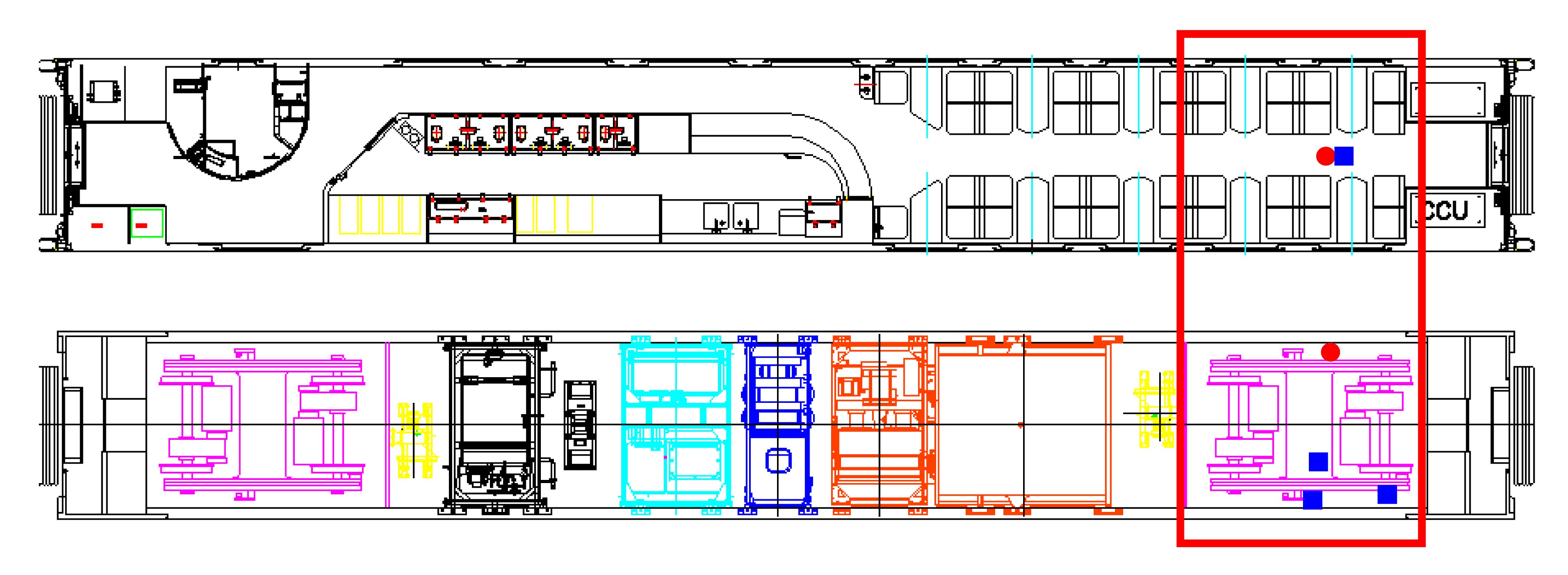
From long-term field experiments on high-speed trains, it was found that wheel polygonal wear caused a series of interior noise problems. These occurred suddenly and seriously, and the railway operation departments of China called these “abnormal interior noise”, but they did not know the mechanism of their productions (Zhang et al., 2013). The present work conducted a typical “abnormal interior noise” analysis. The high-speed train under investigation is made up of 16 coaches and its business operational speed is 300 km/h. The sketch of the coach generating “abnormal interior noise” is shown in Fig. 1.
Fig.1 Measuring points on the high-speed coach generating “abnormal interior noise” The red “●” refers to the acoustic measuring points, and the blue “■” denotes the vibration measuring points
There is a microphone at a vertical height of 1.5 m above the interior floor used for testing the interior noise and a surface microphone installed on the exterior floor for testing the exterior noise. An accelerometer was fixed on the interior floor to measure the vertical vibration of the floor, and three accelerometers were fixed on the axle box, the bogie frame, and the car body, respectively, to measure the vertical vibration of the bogie.
Fig. 2 shows the test photos. Both the noise and the vibration before and after re-profiling were tested, as well as the wheel roughness.
Fig.2 Test photos: (a) surface microphone installed on the exterior floor; (b) wheel roughness measurement
The vibration and acoustic measurements were conducted using a B&K PULSE platform, including a B&K 4190 microphone, a B&K 4948 surface microphone, four B&K 4508 accelerometers, and a B&K Type 3560D data acquisition hardware. The wheel roughness measurement was carried out using a Müller-BBM’s m|wheel.
2.2. Characteristics of wheel diameter difference and polygon
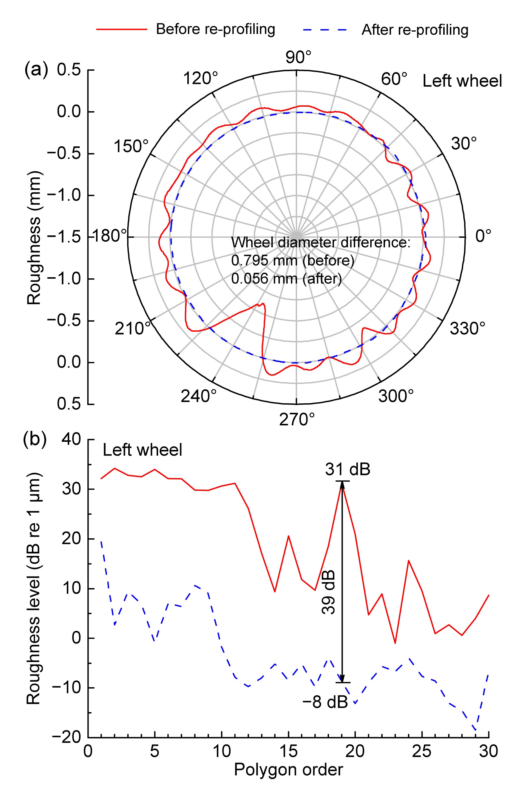
Fig. 3 shows the roughness and the polygon order of the wheel circumference of the left 4th axle of the coach bogie before and after re-profiling. The roughness results (Fig. 3a) are based on the wheel diameter before and after re-profiling.
Fig.3 Wheel roughness and polygon order: (a) wheel roughness; (b) polygon order
From Fig. 3a, it can be seen that the roughness of the wheel before re-profiling is very large. For example, at 240°, the roughness is about −0.573 mm of the wheel before re-profiling, and it is about 0.001 mm after re-profiling. Here, −0.573 mm means its roughness is much bigger than 0.001 mm. The diameter difference of the wheel before re-profiling is up to 0.795 mm. The wheel diameter difference here is defined by
,
where Rmax and Rmin are the maximum and minimum wheel roughness in numerical value, respectively.
The statistical results of wheel roughness tests show that the diameter differences of all other wheels are less than 0.1 mm except the wheels of the 4th axle before re-profiling. After re-profiling, the diameter difference of all the wheels are less than 0.1 mm. Fig. 3b indicates the polygon order distributions corresponding to the measured results as shown in Fig. 3a. In Fig. 3b, the horizontal axis illustrates the polygon order and the vertical axis denotes the amplitudes of the wheel polygons. The peaks mean that the corresponding polygons have a large contribution to the uneven wear of the wheels. Fig. 3b shows the high peak at the ordinate of 19, which indicates that the 19th order polygonal wear of the wheel is very serious. After re-profiling, the roughness level of the 19th order polygon reduced nearly 39 dB.
2.3. Effect of re-profiling on vehicle noise and vibration
Here the train is running at 293 km/h (the actual tested speed). Fig. 4 shows the measured results of noise and vibration before and after re-profiling. Before and after re-profiling with polygonal wear, the acceleration level differences of the axle box, the bogie frame, and the car body reach almost 16–19 dB (Fig. 4a). This phenomenon is particularly obvious on the axle box whose acceleration level decreases from 46 dB to 27 dB. The wheel polygonal wear can cause a very high acceleration level of the axle box. In addition, such a fierce vibration due to the wheel polygonal wear excitation is further transmitted into the coach and the track infrastructure. The acceleration level of the interior floor increases by 7 dB.
Fig.4 Noise and vibration before and after re-profiling: (a) overall levels; (b) 1/3 octave band and FFT
The wheel polygonal wear increases the extra exterior noise in bogie area by 9 dB(A). The big exterior noise and the strong vehicle vibration eventually result in the 11 dB(A) increase of the interior noise (Fig. 4a). The interior noise level directly affects the ride comfort of a high-speed train. In this test, the 11 dB(A) overall level increase of the interior noise is mainly caused by the significant noise components in the 1/3 octave band centred at 500 Hz (Fig. 4b). The sound pressure level in this 1/3 octave band before re-profiling is nearly 19 dB(A) bigger than after re-profiling, and the 1/3 octave band centred at 500 Hz includes those at 447–562 Hz frequencies. In this range, it is found, by fast Fourier transformation (FFT) analysis, that there is the highest peak at 536 Hz as shown in Fig. 4b. Here 536 Hz is just the passing frequency of the 19th order polygon when the train is running at 293 km/h.
For a given train speed v, the passing frequency of the wheel polygon is calculated by
,
where d (d=0.92 m) is the wheel diameter, and i is the polygon order. Hence, the 19th order polygon of the wheel wear can excite the strong wheel/rail vibration and the big noise at about 540 Hz at about 300 km/h.
3. Model of polygonal wheel for wheel/rail rolling noise calculation
From the above, it is clear that the wheel polygonal wear has a major impact on the interior noise and exterior noise of the high-speed train. However, up to now there has been little understanding or research on the effect of the wheel polygonal wear on the interior and exterior noise of high-speed trains, and the wheel/rail rolling noise. The maintenance regulation of China’s high-speed trains now has a criterion of high-speed wheel re-profiling based on wheel diameter difference due to uneven wear, regardless of the wheel polygonal wear characteristics and its mechanisms. The current wheel re-profiling criterion involves only the effect of the wheel uneven wear on the vehicle dynamic performance, but neglects that of the interior noise problem related to the uneven wear characteristics of the wheel. There are two problems with this criterion: (1) the serious uneven wheel wear generally occurs due to the wheel polygonal wear of low order (the low passing frequencies) and high amplitudes, which can cause the annoying interior noise; (2) in spite of mild uneven wheel wear (i.e., not a large wear amplitude), the wheel polygonal wear of high order (high passing frequencies) still creates a large interior noise. If the wheel uneven wear situation is classified as (2) in maintenance, it can avoid re-profiling according to the present criterion. So the re-profiling criteria for high-speed wheels need to involve the effect of the polygonal wear on not only the dynamic behavior but also on the noise of the vehicle.
3.1. Characteristics of two wheels with the same diameter difference
Fig. 5 indicates the measured results of nearly the same diameter difference but the different wheel polygon distributions of the two high-speed wheels, A and B. Fig. 5a shows that the diameter differences of the two wheels are about 0.054 mm. However, their wheel polygonal wear is different (Fig. 5b). In general, the roughness amplitudes of most order polygons of the wheel B are larger than those of the wheel A. However, wheel A shows the 20th order polygonal wear with a high peak, as indicated in Fig. 5b.
Fig.5 Wheel roughness and polygon order: (a) wheel roughness; (b) polygon order
To investigate the noise difference caused by a very similar diameter difference of the high-speed wheels with different polygon distributions, the high-speed wheel-track noise software (HWTNS) is used to analyze wheel/rail noise of the two wheels running at 300 km/h.
3.2. Theory of wheel/rail rolling noise prediction
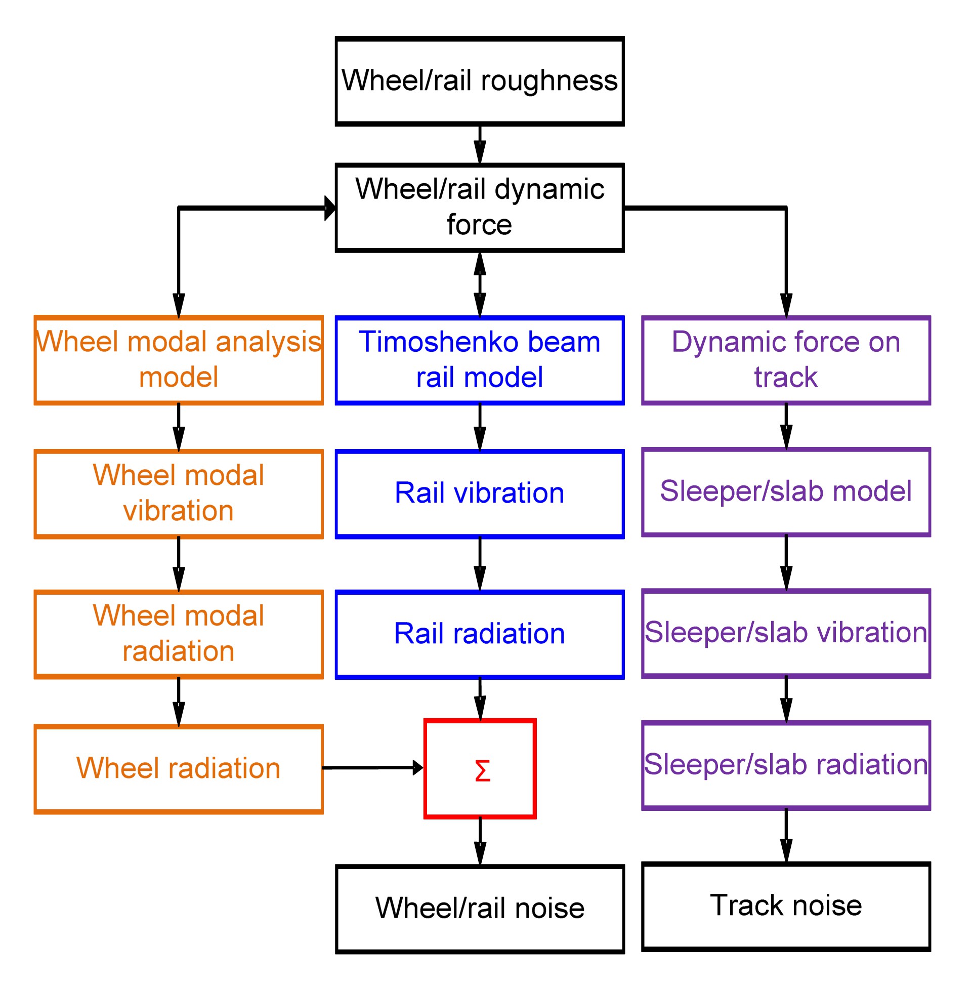
The HWTNS was developed by Wu and Thompson (1999; 2000; 2001). It uses a similar conformation to the track-wheel interaction noise software (TWINS) (Thompson et al., 1996a; 1996b), but adds the ballastless track model of high-speed railway (Wu, 2012). Fig. 6 shows the flow chart of the HWTNS.
Fig.6 Wheel/rail noise prediction using the HWTNS (Wu, 2012)
For the ballastless track model in the HWTNS, a wheel/rail interaction model is used to calculate wheel/rail dynamic force based on wheel/rail combined roughness. This dynamic force has effects on the rolling contact of the wheel and the rail and causes the vibration and the noise radiation. The dynamic force can also transmit to the track infrastructure through the rails and fasteners, which causes vibration and noise radiation of the sleepers or slabs. More details are given in (Wu, 2012).
The vibration and sound radiation of the wheel is calculated using a semi analytical method. They are divided into three parts, namely vibration and sound radiation caused by (i) wheel axial modes, (ii) wheel radial modes, and (iii) wheel rim rotation modes. The overall sound power level of the wheel is obtained by the summation of the sound radiation of each mode (Thompson, 1997):
,
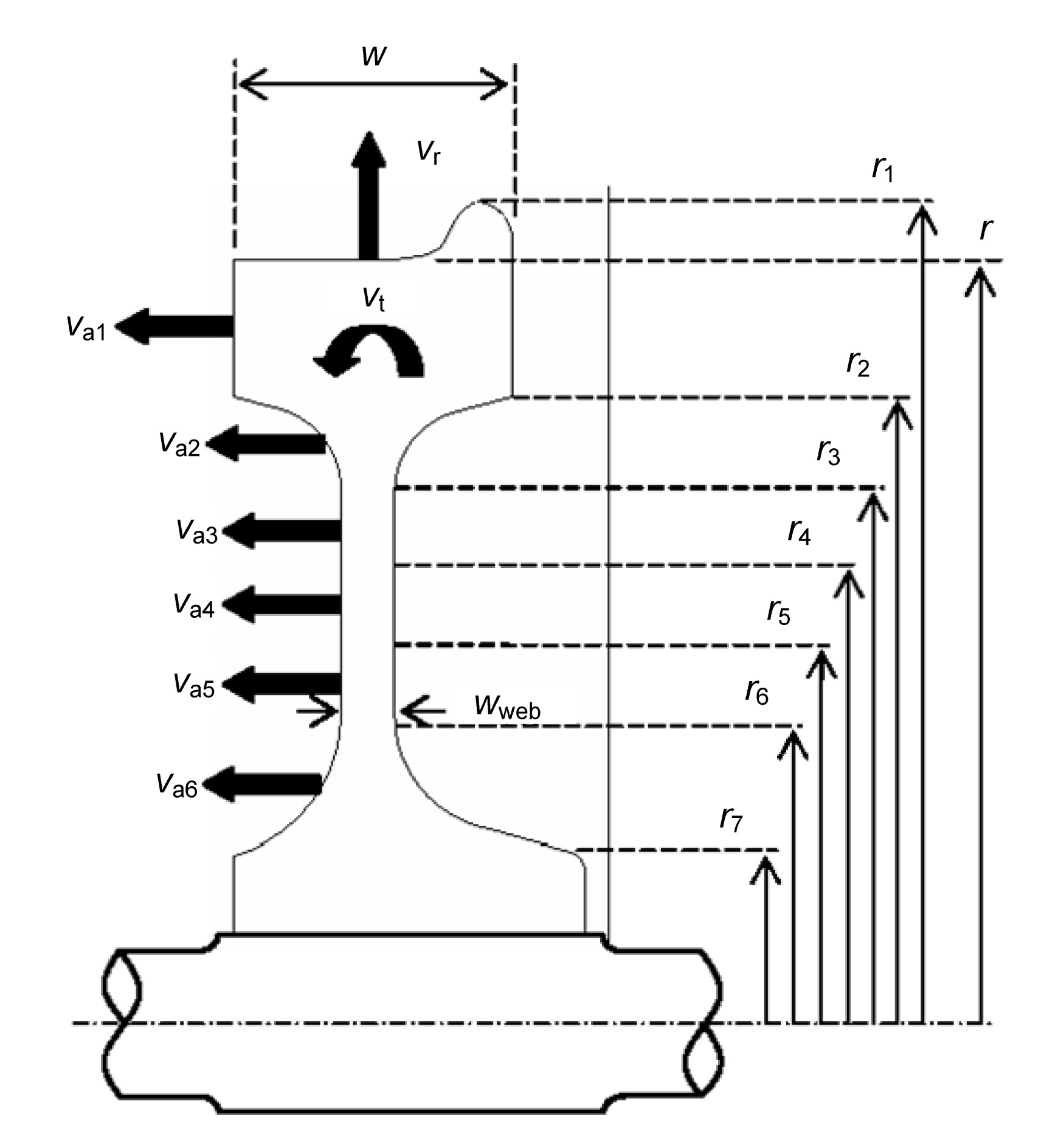
where ρ is the density of the air and c is the sound velocity in the air. σa(n), σr(n), and σt(n) are the sound radiation ratios of the wheel axial vibration, the wheel radial vibration, and the wheel rim rotation of n nodal diameter, respectively. , , and are the mean square velocities of the wheel axial vibration, the wheel radial vibration, and the wheel rim rotation of n nodal diameter, respectively. Saj, Sr, and St are the sound radiation areas of these mean square velocities, respectively. For the wheel axial vibration, the area of the wheel web is large and its velocity generates great variation, so in the calculation of the vibration and sound radiation of the wheel it needs to be divided into circles with different radii and then the vibration and sound radiation of the circles are summed.
Fig. 7 shows the divided circles of the wheel in the HWTNS.
Fig.7 The divided circles of the wheel in the HWTNS (Wu, 2012)
The sound radiation areas are given by Thompson (1997):
,
,
,
where r is the radius of the wheel, rj (j=1, 2, …, 7) is the radius of each divided circle, w is the width of the wheel tire in its cross-section, and wweb is the width of the wheel web in its cross-section (Fig. 7).
The sound radiation ratio of each nodal diameter mode is given by Thompson (1997):
(i) Wheel axial vibration
(ii) Wheel radial vibration
(iii) Wheel rim rotation
where f is the frequency. and fca, fcr, and fct are the critical frequencies when the bending wavelength of the wheel vibration and the acoustic wavelength are equal.
The rail is defined as the infinite line sound source and its radiation is given by Wu (2012):
,
where L is the length of the rail, h is the length of the rail cross-section profile in the vertical projection, and σr is the rail sound radiation ratio. is the mean square velocity of vertical vibration of the rail and is given by
,
where vr is the vertical velocity of the rail in the length of Δz.
The slab sound radiation is given by Wu (2012):
where is the mean square velocity of vertical vibration of the slab in the track length of L, Lp is the length of the slab, and B is the width of the half slab. When the slab is considered as a rigid body, the mean square velocity of vertical vibration of the slab in Eq. (12) is given by
where is the mean square velocity of vertical vibration of single slab, Np is the quantity of the slabs in the track length of L, and vci and are the vertical velocity of the slab mass center and the rotational velocity around its mass center, respectively.
Predicting the wheel/rail noise using the HWTNS needs three input files including wheel data, wheel/rail combined roughness, and rail sound radiation ratio. The wheel data is analyzed using the wheel finite element (FE) model based on the commercial ANSYS. The wheel/rail combined roughness is calculated using the method described in (Thompson et al., 1996a; 1996b). The rail roughness is the Class A selected from the HARMONOISE project (van Beek and Verheijen, 2003). The rail sound radiation ratio calculation uses the data of UIC 60 rail.
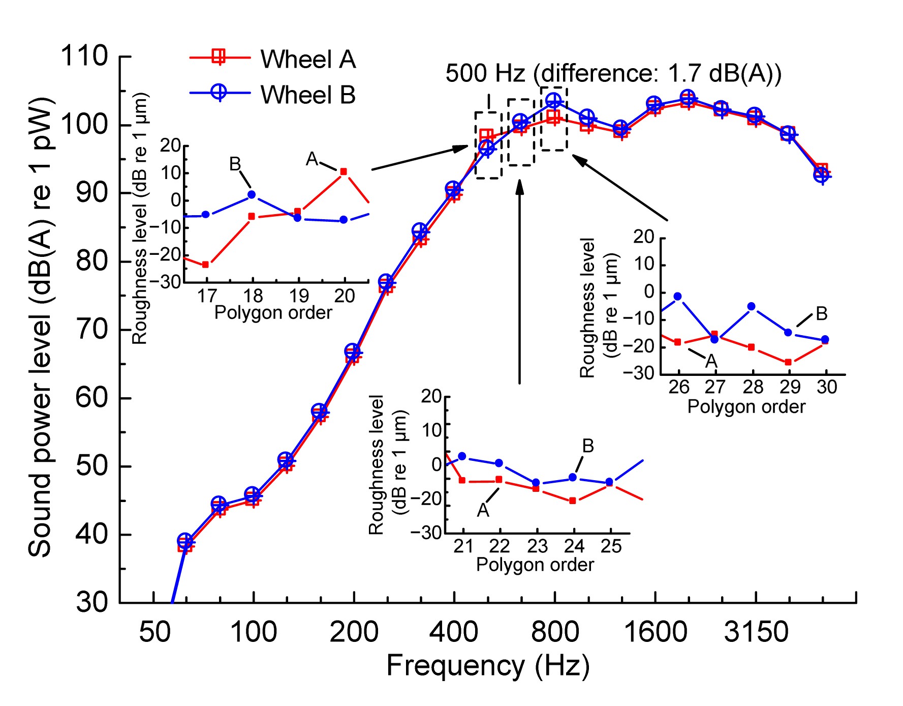
Fig. 8 shows the wheel/rail noise prediction results of wheel A and wheel B at 300 km/h.
Fig.8 Sound power level of wheel/rail noise
From Fig. 8, it can be seen that the sound power levels of wheel B and the rail in rolling contact are higher than that of the wheel A and the rail in all 1/3 octave bands except for one band centred at 500 Hz. It is because the roughness amplitudes of most order polygons of the wheel B are higher than those of wheel A, but the peak of the 20th order polygon of wheel A is very prominent (Fig. 5b, also see the small picture on the left in Fig. 8). When the train operates at 300 km/h, the 20th order polygon of the wheel would excite vibration with frequency at about 577 Hz, which is in the 1/3 octave band centred at 630 Hz. However, the simulation result (Fig. 8) shows that the sound power level of wheel A and the rail is higher than that of wheel B and the rail in the 1/3 octave band centred at 500 Hz, not 630 Hz. The reason for this 1/3 octave frequency band difference is attributed to the correspondence between the wavelengths and the frequencies in the wheel/rail noise calculation. Table 2 shows the difference of 1/3 octave frequency bands between the simulated and actual cases.
Table 2
The difference of 1/3 octave frequency bands between the simulated and actual cases
Polygon order
Actual case
Simulated case
Frequency (Hz)
1/3 octave frequency band (Hz)
Wavelength (m)
1/3 octave wavelength band (m)
1/3 octave frequency band (Hz)
13
375.01
400
0.2222
0.2
400
14
403.86
400
0.2063
0.2
400
15
432.71
400
0.1926
0.2
400
16
461.55
500
0.1806
0.2
400
17
490.40
500
0.1699
0.16
500
18
519.25
500
0.1605
0.16
500
19
548.09
500
0.1520
0.16
500
20
576.94
630
0.1444
0.16
500
21
605.79
630
0.1376
0.125
630
22
634.63
630
0.1313
0.125
630
23
663.48
630
0.1256
0.125
630
24
692.33
630
0.1204
0.125
630
25
721.18
800
0.1156
0.125
630
As shown in Table 2, when the train operates at 300 km/h, the actual excitation (passing) frequencies of the 13th–25th order polygons of the wheel and their 1/3 octave frequency bands are shown, and their correspondences used in the numerical simulation are also shown. In the wheel/rail noise calculation (in the HWTNS), part of the input data is the wheel/rail combined roughness in 1/3 octave frequency band (some of the bands are as indicated in Table 2). So the FFT analysis on the measured wheel circle irregularity samples is first carried out to translate them to the samples expressed with different wavelengths. Then the different wavelengths are allocated into several 1/3 octave wavelength bands (Table 2, and Eqs. (20) and (21)), and further transformed into 1/3 octave frequency bands at the specific speed (300 km/h). Obviously, the wavelength of the 20th order polygon is 0.1444 m which belongs to the 1/3 octave wavelength band centered at 0.16 m, and this 1/3 octave wavelength band is transformed into 1/3 octave frequency band centered at 500 Hz (not 630 Hz) at 300 km/h. That is the root cause of the 1/3 octave frequency band difference between the numerical simulation and the actual result of the 20th order polygon. In addition, the wavelength 0.1444 m of the 20th order polygon is just the lower boundary value of the 1/3 octave wavelength band centered at 0.16 m, and neighbors the 1/3 octave wavelength band centered at 0.125 m. During the transformation from the measured wheel circle irregularity samples to the wavelength samples through the FFT analysis, the partial power of the 20th order polygon leaks into the 1/3 octave wavelength band centred at 0.125 m (corresponding to 630 Hz) though it belongs to the 1/3 octave wavelength band centred at 0.16 m (corresponding to 500 Hz). Therefore, in spite of the visible 20th order polygon occurring on wheel A, the wheel/rail rolling noise calculation results in the 1/3 octave band centred at 500 Hz and is only a little higher than that of the wheel B.
The sound power levels of wheel B in the 1/3 octave bands centred between 630 Hz and 800 Hz are much higher than those of wheel A owing to the larger roughness of the 21st to the 25th and the 26th to the 30th order polygons (see the small pictures at the bottom and in the right of Fig. 8, respectively).
In summary, although there are some differences between the actual data and the calculated sound power levels of the wheel polygons in 1/3 octave frequency bands, the calculation results can still show well the characteristics of the wheel polygon excitation at high-speed. The overall sound power levels of wheel A and wheel B are 110.9 dB(A) and 111.6 dB(A), respectively. It can be seen that a very similar wheel diameter difference can cause different wheel/rail rolling noises because of different distribution of the wheel polygon order.
4. Prediction model of interior noise of coach
To further study the influence of wheel polygonal wear on the interior noise of a high-speed train, the simulation model of the coach end is built up by means of the vibro-acoustic analysis software VA One 2012. The model is developed based on a hybrid of the finite element method and the statistic energy analysis (Langley and Bremner, 1999; Shorter and Langley, 2005; Cotoni et al., 2007), which is called the hybrid FE-SEA for short.
4.1. Theory of the hybrid FE-SEA
The FE method and the SEA are at present the two main methods for solving the acoustic problem of complex structural systems. The FE method usually works well in solving the structural acoustic problem in the low frequency range, where the modal density is low and the system exhibits a global modal behavior. The SEA is usually used for solving the acoustic problem of complex structural systems at high frequencies, where the modal densities of all the subsystems are very high. For the high-speed train, because its large size leads to the generation of numerous elements in modeling the coach for solving its noise problem, it is difficult to solve the vibro-acoustic issue only using the FE method. Furthermore, the coach interior noise caused by wheel polygonal wear is always prominent in the middle frequency range, which is defined as from about 200 Hz to 1000 Hz in the present analysis (Fig. 4b). So the hybrid FE-SEA is used in the noise calculation.
However, the coupling of FE and SEA in a single model is difficult because the two methods differ in two ways: (i) the FE method is based on dynamic equilibrium while the SEA is based on the conservation of energy flow, and (ii) the FE method is a deterministic method while the SEA is an inherently statistical method. Here the two main equations of the hybrid method are given as follows (Shorter and Langley, 2005; Cotoni et al., 2007):
,
,
where
,
,
.
The definitions of the variables in Eqs. (14)–(18) can be found in (Langley and Bremner, 1999; Shorter and Langley, 2005; Cotoni et al., 2007). Eq. (14) represents the subsystem energy balance in the SEA, in which is the external power input, and Eq. (15) describes the system response by the FE method, while Sqq is the ensemble average cross-spectral response. Eqs. (14)–(18) couple the FE with the SEA. Eq. (14) has a precise form of the SEA, but the coupling loss factor ηjk and the loss factor ηd,j are calculated using the FE model. Furthermore, Eq. (15) has the form of a standard random FE analysis, but additional forces arise from the reverberant energies in the SEA subsystems. If the SEA subsystems are not included, it is obvious that the present hybrid method is just the FE method. On the other hand, if only the junctions between the SEA subsystems are modeled by the FE method, the hybrid method becomes the SEA method.
4.2. Interior noise simulation model of the coach end
The hybrid FE-SEA simulation model of the high-speed coach end includes the beam, the plate, and the acoustic cavity subsystems. Fig. 9 presents the hybrid model in VA One 2012.
Fig.9 The hybrid FE-SEA simulation model of coach end
Because the modal densities of the beam subsystems are very low, the beam subsystems are meshed into the subsystems characterized by the FE models. The noise sources, including the wheel/rail noise and the aerodynamic noise, are extracted from the field pass-by test data of the high-speed trains operating at 300 km/h. In the test, B&K 4948 surface microphones are fixed on the external floor above the bogie and on the external side wall of the car body. So the wheel/rail noise and the aerodynamic noise are treated approximately as the diffuse acoustic field (DAF) loaded on the plate. Transmission loss (TL) data, including from the floor, the side wall, and the roof, is taken from the test results in the acoustics laboratory, and defined through the area junction. A semi-infinite fluid (SIF) is created and connected to the car body to simulate the outside acoustic environment.
Fig. 10 shows the interior noise results of the numerical simulation and the field experiment, including before and after re-profiling. In the simulation, the different cases change only the wheel/rail noise inputs.
Fig.10 Results of the numerical simulation and the experiment before (a) and after (b) re-profiling
From Fig. 10, it can be seen that both before and after re-profiling, the interior acoustic energy is dominant in the frequency range from 200 Hz to 2000 Hz, which belongs to the middle frequency range. The predicted responses and the measured sound pressure level are generally in good agreement. The difference of the overall sound pressure level is less than 2 dB(A). Thus, the interior noise hybrid FE-SEA model established in this study is reliable and effective. However, in the low frequency range (frequencies lower than 200 Hz), simulation results do not agree well with experimental results. This is because the hybrid FE-SEA model is more suitable for the mid-frequency. For low-frequency, simulation results could be improved by the use of a boundary element method (BEM) fluid and a set of plane waves. Further investigation on this topic is being conducted.
The wheel polygons which are going to be discussed have the characteristics of high order polygons (13 to 30). They can excite strong vibration with frequencies from 375 Hz to 865 Hz (at 300 km/h), which are typical mid-frequency. So in the following sections, the hybrid model is used to calculate the effect of different wheel polygon characteristics on the coach interior noise. We examine different wheel/rail noise sources due to different wheel polygon characteristics.
5. Influence of different wheel polygonal wear on noise
5.1. Characteristics of wheel polygon
Usually, the wheel polygonal wear has three characteristics, which should be discussed before carrying out the analysis. They are (i) the different polygon order with very similar roughness levels, (ii) very similar polygon order with different roughness levels, and (iii) very similar polygon order and very similar roughness levels with different distribution phases of the polygons. These characteristics can be found from the detailed analysis of the measured wheel circle irregularity data.
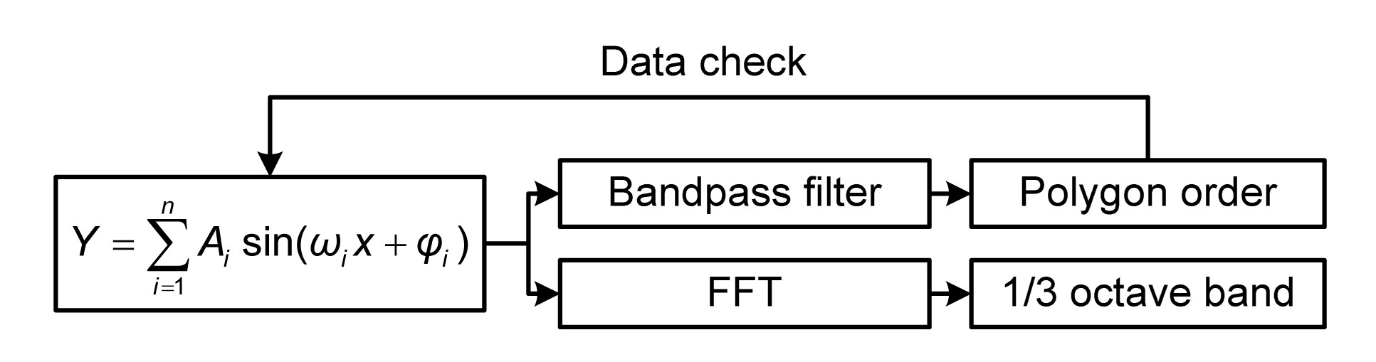
A MATLAB program is developed to construct a series of different wheel polygons. The code technique routine is indicated with Fig. 11.
Fig.11 The MATLAB code technique routine for creating wheel polygon data
The created wheel circle irregularity sample consists of a series of sine curves, Aisin(ωix+φi) (i=1, 2, …, n), where Ai is the roughness amplitude of wave i, ωi is the wavenumber and φj is the phase angle. First, use a bandpass filter (here we use the Chebyshev filter (Williams and Taylors, 2006)), which filters out each polygon and obtains its roughness level. Then all filtered wheel circle irregularity samples are summed and these samples correspond to their polygon order. It is checked whether the summed sample is correct for the original sample. If not, the bandpass filter should be redesigned. In addition, the FFT analysis can translate wheel circle irregularity samples into wavenumber samples using
.
Eq. (19) implements the transform given for vectors of length N, where ωN=e(2πi)/N, which is the Nth root of the unit.
Through FFT analysis, the 1/3 octave wavelength band can be calculated. The relationship between the centre wavelength and the cut-off wavelength of 1/3 octave is given by
,
,
where λupper, λlower, and λc are the upper cut-off wavelength, the lower cut-off wavelength, and the centre wavelength, respectively, where n=1/3 represents a 1/3 octave.
5.2. Effect of different order of wheel polygon on noise
According to the extensive investigation into high-speed wheel roughness and vehicle noise, mainly the 19th and the 20th order wear polygons are those which quite often cause serious noise problems. To study the influence of different polygon order of the worn wheels, a MATLAB program is used to generate polygon wheel shapes with order from 13 to 30. Their roughness levels are 30 dB.
Fig. 12a shows the different polygons vs. their order, and Fig. 12b shows their roughness levels vs. their wavelengths.
Fig.12 Different polygon order: (a) polygon roughness levels characterized by order; (b) polygon roughness levels characterized with the wavelength
Although there are 18 polygon order (Fig. 12a), there are only four main peaks with different wavelengths in 1/3 octave (Fig. 12b). The root cause of this phenomenon has already been discussed in Section 3.3 (Table 2). Because noise peaks are mainly due to wheel polygon peaks (there are only four main peaks as indicated in Fig. 12b), and to avoid some critical polygon order (Table 2), the 15th, the 19th, the 24th, and the 30th order polygons are selected in calculating the effect of them on wheel/rail noise and interior noise using the models described in the Sections 3 and 4.
Figs. 13a and 13b indicate the effect of different polygon order on the wheel/rail noise and the interior noise at 300 km/h, respectively.
By using the obvious wheel polygons as inputs in the calculation, there are four peak frequencies of 400 Hz, 500 Hz, 630 Hz, and 800 Hz in the calculated noise results. The noise peak frequencies correspond to the wheel polygon order. Notably, even though the roughness levels are 30 dB (Fig. 12a) and the peak amplitudes with different wavelengths are almost the same (Fig. 12b), the wheel/rail noise levels caused by the four different order polygons are different. As the wheel polygon order increases, in the different 1/3 octave bands, the wheel/rail noises increase by about 5 dB(A) per 1/3 octave. This is mainly because the higher order polygon has the higher passing frequency (corresponding to the shorter wavelength) and a larger excitation energy when the wheel rolls over the rail at the same speed, compared to the lower order polygon with the same roughness level. The other reason for this phenomenon is that as the excitation frequencies increase, the sound radiation ratios of both the wheel and the rail increase. Generally speaking, the higher sound radiation ratio causes the higher sound radiation power. Thus, although there are the same roughness levels, different polygon order can cause different wheel/rail noises. Therefore, the higher order polygon can cause the higher wheel/rail noise level.
From Fig. 13b, there are four peak frequencies in the interior noise, which is the same as in the wheel/rail noise. So the wheel/rail noise makes a great contribution to the interior noise. However, the increase in the ratio of the interior noise at the peak frequencies is different from that of the wheel/rail noise (as indicated in Fig. 13a). One reason for this phenomenon is that the interior noise is influenced by not only the wheel/rail noise, but also other exterior sources and the structure TL.
Fig.13 Different polygon order: (a) wheel/rail noise; (b) interior noise
5.3. Effect of different roughness levels of wheel polygon on noise
With increase in operational mileage, the roughness levels and the distribution of the wear polygons will change. Here this section discusses the influence of different roughness levels of the wear polygon on the noise level. Taking the frequently occurring wheel polygon order (the 19th order polygon) as a numerical example, in which the MATLAB code discussed above is used to make it with different roughness levels. Fig. 14a shows the 19th order polygon with different roughness levels, characterized by order, and Fig. 14b shows the roughness level described with the wavelength.
Fig.14 Different roughness levels: polygon roughness levels characterized by order (a) and with the wavelength (b)
The roughness levels of the 19th order polygon increase from 21 dB to 39 dB with a 3 dB interval, as indicated in Fig. 14a. The roughness levels in the 1/3 octave wavelength centred at 0.16 m also increase with about 3 dB interval, as indicated in Fig. 14b.
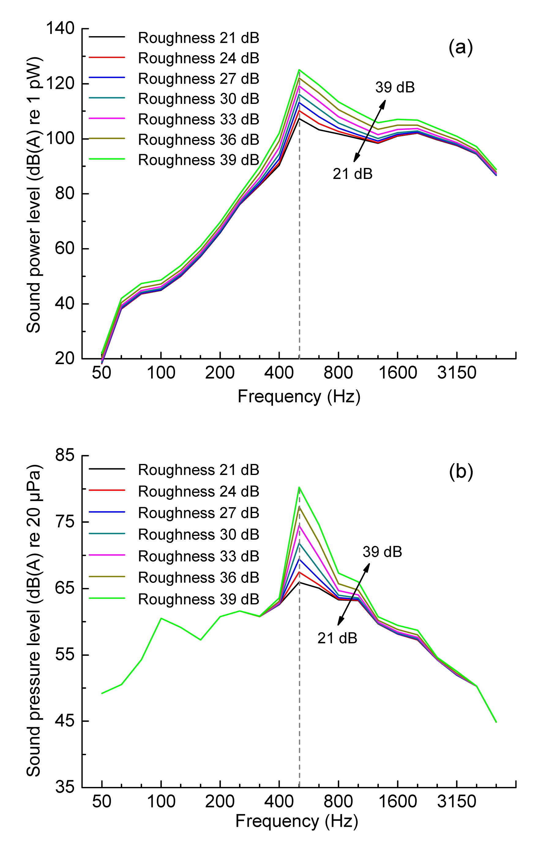
Fig. 15 shows the results of the wheel/rail noise and the interior noise at 300 km/h.
Fig.15 Different roughness levels: (a) wheel/rail noise; (b) interior noise
Obviously, there is a peak frequency of 500 Hz in the wheel/rail noise that is the passing frequency of the 19th order polygon at 300 km/h. As the roughness level of the polygon increases from 21 dB to 39 dB with a 3 dB interval, the wheel/rail noise in the 1/3 octave band centred at 500 Hz increases from 107 dB(A) to 125 dB(A) also with about a 3 dB interval (Fig. 15a).
As shown in Fig. 15b, there is a 500 Hz peak frequency in the interior noise which is the same as in the wheel/rail noise. With the increase of the roughness level of the 19th order polygon, the interior noise in the 1/3 octave band centred at 500 Hz increases from 66 dB(A) to 80 dB(A), but with a nonlinear increase.
5.4. Effect of different phases of wheel polygon on noise
As shown in Sections 5.2 and 5.3, both the different order polygons and the different roughness levels have a great effect on the interior noise. Actually, the different polygon phases are also important, especially for the re-profiling. This is because the different polygon phases can be combined to make different wheel diameter differences even though the order distribution and roughness of the wheel polygons are the same. In other words, high order wheel polygons, which can make the annoying interior noise, may occur with normal or low wheel diameter difference. To study the influence of the different polygon phases on the interior noise, this section discusses whether the present standard of wheel re-profiling is suitable for the noise reduction problem, being only based on the diameter difference. We consider the 17th to 19th order polygons and the different diameter differences are obtained by creating different combinations of the polygon phases.
Using three sine curves creates the different combinations of the different polygon phases. The equation including the three sine waves is given by,
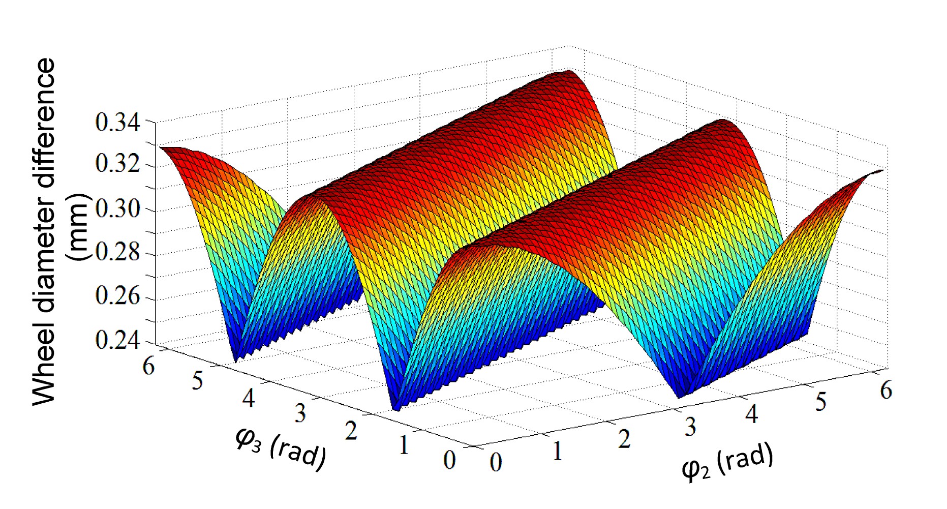
where A, B, and C are used to define the roughness levels of the 17th, the 18th, and the 19th order polygons, respectively. ωj (j=1, 2, 3) is used to indicate the jth order polygon and φj (j=1, 2, 3) is used to denote the phase angle of the jth order polygon. Ymax−Ymin is the wheel diameter difference. To make the diameter difference higher than 0.3 mm which is caused by the combination of the three polygons described with Eq. (22), the calculation uses the 30 dB roughness level of the 17th order polygon and 33 dB roughness levels of both the 18th and the 19th order polygons. Here 0.3 mm is the upper limit of the wheel diameter difference according to the maintenance standard for the high-speed trains of China (Zeng, 2011). The numerical analysis sets φ1=0 rad while φ2 and φ3 change from 0 rad to 2π rad. Fig. 16 shows the effect of the variations of φ2 and φ3 on the wheel diameter differences with φ1=0 rad.
Fig.16 Wheel diameter differences caused by combination of different phase angles
From Fig. 16, it can be seen that even though the roughness levels of the wheel polygons do not change, their different phases can be combined to make the different wheel diameter differences. When φ1=φ2=φ3=0 rad, there is the biggest diameter difference at 0.33 mm. When φ1=0 rad, φ2=4.54 rad, and φ3=5.93 rad, there is the smallest diameter difference, 0.24 mm. The difference between the biggest and the smallest is about 0.1 mm.
Fig. 17 shows the wheel/rail noise and the interior noise of the two cases at 300 km/h which indicate the biggest and the smallest diameter differences (indicated by Max and Min in the figure) discussed above.
Fig.17 Different polygon phases: (a) wheel/rail noise; (b) interior noise
As shown in Fig. 17a, there is a peak frequency at 500 Hz in the wheel/rail noise as the 17th to 19th order polygons have an excitation frequency in the 1/3 octave band centred at 500 Hz. In spite of the different polygon phases (different diameter difference), their wheel/rail noise sound power levels in the 1/3 octave frequency centred at 500 Hz are nearly the same. Thus, the polygon phase’s change cannot change its wheel/rail noise level in the excitation frequency band. However, there are some differences between the wheel/rail noises of the two cases in the 1/3 octave bands below 500 Hz and above 1000 Hz. These are due to the differences between their wavelength spectra which are caused by the characteristic of the filter in the program. Because the wheel/rail noises in the 1/3 octave band centred at 500 Hz are almost the same, there is little difference between the overall levels of these two cases.
From Fig. 17b, it can be seen that there is also little difference between the interior noises, similar to the wheel/rail noises. Nevertheless, the interior noise in the 1/3 octave bands below 500 Hz are nearly the same which is a little different from the wheel/rail noise. That is because wheel/rail noise in the 1/3 octave bands below 500 Hz is not as important as other exterior sources. The overall sound pressure levels of the interior noises are nearly the same in the two cases. So the influence of the polygon phases on interior noise is small.
However, the maintenance regulation of China’s high-speed train now uses a criterion for re-profiling based only on diameter difference, regardless of the wheel polygonal wear status. It is generally considered that when the wheel circle diameter difference is smaller than 0.1 mm, the polygon status is good. When the diameter difference due to the polygonal wear is between 0.1 mm to 0.2 mm, it is normal. Furthermore, when the diameter difference is bigger than 0.3 mm, it is bad. If the diameter difference is bigger than 0.3 mm, the wheel needs to be re-profiled (Zeng, 2011). Although the interior noise is almost the same for the above two cases, the wheel with 0.33 mm diameter difference needs to be re-profiled and the other wheel with 0.24 mm diameter difference could continue working.
From the test and simulation results shown in Section 3, we find that although the wheel circle diameter differences are nearly the same, different wheel polygons can cause different wheel/rail noise levels. Furthermore, we can find that even if the wheel polygon order are the same, their different polygon phases can be combined to make a different wheel circle diameter difference. However, the wheel/rail noise, especially the interior noise, is more determined by the order of the wheel polygons, not the phase of wheel polygons. In summary, a criterion based on only the wheel diameter difference is not suitable for carrying out re-profiling for noise reduction. The wheel polygon characteristics should also be considered.
6. Conclusions
The present work conducts a detailed investigation into the relationships between high-speed wheel polygonal wear and wheel/rail noise, and the interior noise of high-speed trains through extensive field experiments and numerical simulations. The conclusions can be drawn:
The field experiments show that when the 19th order polygonal wear is prominent and common, the vibration and noise of the high-speed coach are dominant at about 540 Hz. That is just the passing frequencies of the 19th order polygon at about 300 km/h. The root cause of the 19th order polygonal wear has not so far been understood. Further investigation is underway on this topic and is not in the scope of this paper.
Through test and simulation, in cases where the wheel circle diameter differences due to the wheel polygonal wear are nearly the same, the different wheel polygonal wear patterns can cause different wheel/rail noise levels.
The numerical simulation shows that different polygon order with nearly the same roughness levels can cause different wheel/rail noise levels and interior noise levels. Namely, the wheel polygons with higher order can make more serious wheel/rail noise and interior noise. This is because the higher order has the higher passing frequency at a certain operational speed, and generates higher wheel/rail vibration energy.
Changing the phases or the distribution of the wheel polygons can change the wheel diameter difference caused by the wheel polygonal wear. However, the effect of the change of the polygon phases is not great on wheel/rail noise and interior noise.
The criterion for re-profiling of high-speed trains needs to involve not only the wheel diameter difference due to the wear but also the characteristics of the wheel polygons.
Acknowledgements
The authors are grateful for Da-bin CUI, Wei LI, Shuo-qiao ZHONG, Heng-yu WANG, and Yong-guo DENG (Southwest Jiaotong University, China) for their assistance in this study.
[1] Behr, W., Cervello, S., 2007. Optimization of a wheel damper for freight wagons using FEM simulation. , Proceedings of the 9th International Workshop on Railway Noise, Munich, 334-340. :334-340.
[2] Bouvet, P., Vincent, N., Coblentz, A., 2000. Optimization of resilient wheels for rolling noise control. Journal of Sound and Vibration, 231(3):765-777.
[3] Cotoni, V., Shorter, P., Langley, R., 2007. Numerical and experimental validation of a hybrid finite element-statistical energy analysis method. The Journal of the Acoustical Society of America, 122(1):259-270.
[4] Jin, X.S., Wu, L., Fang, J.Y., 2012. An investigation into the mechanism of the polygonal wear of metro train wheels and its effect on the dynamic behaviour of a wheel/rail system. Vehicle System Dynamics, 50(12):1817-1834.
[5] Johansson, A., 2006. Out-of-round railway wheels-assessment of wheel tread irregularities in train traffic. Journal of Sound and Vibration, 293(3-5):795-806.
[6] Johansson, A., Andersson, C., 2005. Out-of-round railway wheels—a study of wheel polygonalization through simulation of 3D wheel/rail interaction and wear. Vehicle System Dynamics, 43(8):539-559.
[7] Jones, C.J.C., Thompson, D.J., 2000. Rolling noise generated by railway wheels with visco-elastic layers. Journal of Sound and Vibration, 231(3):779-790.
[8] Langley, R.S., Bremner, P., 1999. A hybrid method for the vibration analysis of complex structural-acoustic systems. The Journal of the Acoustical Society of America, 105(3):1657-1671.
[9] Meinke, P., Meinke, S., 1999. Polygonalization of wheel treads caused by static and dynamic imbalances. Journal of Sound and Vibration, 227(5):979-986.
[10] Morys, B., 1999. Enlargement of out-of-round wheel profiles on high speed trains. Journal of Sound and Vibration, 227(5):965-978.
[11] Nielsen, J.C.O., Johansson, A., 2000. Out-of-round railway wheels—a literature survey. Proceedings of the Institution of Mechanical Engineers, Part F: Journal of Rail and Rapid Transit, 214(2):79-91.
[12] Nielsen, J.C.O., Lunden, R., Johansson, A., 2003. Train-track interaction and mechanisms of irregular wear on wheel and rail surface. Vehicle System Dynamics, 40(1-3):3-54.
[13] Shorter, P.J., Langley, R.S., 2005. Vibro-acoustic analysis of complex systems. Journal of Sound and Vibration, 288(3):669-699.
[15] Thompson, D.J., Gautier, P.E., 2006. Review of research into wheel/rail rolling noise reduction. Proceedings of the Institution of Mechanical Engineers, Part F: Journal of Rail and Rapid Transit, 220(4):385-408.
[16] Thompson, D.J., Hemsworth, B., Vincent, N., 1996. Experimental validation of the TWINS prediction program for rolling noise, Part I: descrisption of the model and method. Journal of Sound and Vibration, 193(1):123-135.
[17] Thompson, D.J., Fodiman, P., Mahe, H., 1996. Experimental validation of the TWINS prediction program for rolling noise, Part II: results. Journal of Sound and Vibration, 193(1):137-147.
[18] van Beek, A., Verheijen, E., 2003. Definition of Track Influence: Roughness in Rolling Noise. Harmonoise Report, HAR12TR-020813-AEA10, the Netherlands :
[21] Wu, T.X., Thompson, D.J., 1999. A double Timoshenko beam model for vertical vibration analysis of railway track at high frequencies. Journal of Sound and Vibration, 224(2):329-348.
[22] Wu, T.X., Thompson, D.J., 2000. Theoretical investigation of wheel/rail non-linear interaction due to roughness excitation. Vehicle System Dynamics, 34(4):261-282.
[23] Wu, T.X., Thompson, D.J., 2001. Vibration analysis of railway track with multiple wheels on the rail. Journal of Sound and Vibration, 239(1):69-91.
[24] Zeng, J., 2011. The Failure Mechanism and Optimization of High-speed Wheel/Rail in Rolling Contact. Technical Report of National Basic Research Program (973) of China, No. 2007CB714702, (in Chinese), Chengdu :
[25] Zhang, J., Xiao, X.B., Han, G.X., 2013. Study on abnormal interior noise of high-speed trains. , Proceedings of the 11th International Workshop on Railway Noise, Uddevalla, Sweden, 691-698. :691-698.
Open peer comments: Debate/Discuss/Question/Opinion


 ORCID:
Open peer comments: Debate/Discuss/Question/Opinion
<1>